View factor derivation - Partially visible disk with oriented area element in normal direction from center
This post is a continuation of the last one View factor - fully visible. We want to compute the view factor of a disk and an oriented differential area located along the disk’s normal. Before, we assumed all of the disk to be visible from our surface. But if our surface is rotated enough, the infinite plane it lies on intersects the disk. The cut off part is then behind the surface, so there is no radiation transfer. We will now handle that case. As before, we will derive the formula given in http://www.thermalradiation.net/sectionb/B-13.html. First a sketch of the updated setup:
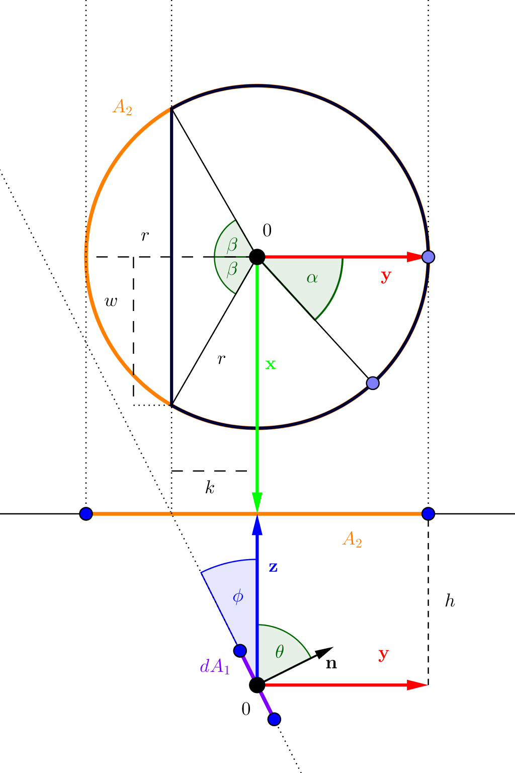
The update from the last post is that we cut off the part of the disk behind the plane. The resulting shape is outlined in the very dark blue.
We will now find the condition for when the disk is fully visible. From the image, we can see that it is fully visible, if \(k\) is larger than the disk’s radius \(r\). Since the normal is perpendicular to the plane, we have \(\phi = \frac{\pi}{2} - \theta\). Computing the tangent yields:
\[\begin{aligned} \tan \phi &= \tan (\frac{\pi}{2} - \theta) \\ &= \cot \theta \\ &= \frac{k}{h} \end{aligned}\]And following from that
\[k = h\cot \theta\]For the visibility condition:
\[\begin{aligned} r \leq k \\r \leq h\cot \theta \\ \frac{r}{h} \leq \cot \theta \\ \cot^{-1}(\frac{r}{h}) \geq \theta \\ \cot^{-1}(\frac{1}{H}) \geq \theta \end{aligned}\]The last line uses the definition \(H = \frac{h}{r}\). The reversal of the inequality sign comes from the fact, that the inverse cotangent function is monotonically decreasing. This is the same condition as given in the reference. If it holds, we can apply the previous post’s reasoning and are finished.
For the next steps we will compute \(\beta\).
\[\begin{aligned} \cos \beta &= \frac{k}{r} \\ &= \frac{h\cot \theta}{r}\\ &= H\cot \theta \\ \beta &= \cos^{-1}(H\cot \theta) \end{aligned}\]Since we will need it later, we can derive another useful expression with the identity \(\sin(\cos^{-1}x) = \sqrt{1-x^2}\)
\[\begin{aligned} \sin \beta &= \sin \cos^{-1}(H\cot \theta) \\ &= \sqrt{1-H^2\cot^2\theta} \\ &= X \end{aligned}\]We will now proceed with the actual computation. It will be split into two parts, since the contour can be decomposed into two parts: A circle segment and a straight line.
Circle segment
Pretty much all the setup is the same as in the last post View factor - fully visible, so I will refer to that for more information. The only difference is the interval over which to integrate. Before we had the full circle in \([0,\pi]\). Now a part is missing. The new interval goes up to \(\pi - \beta\) and starts at that value in negative \(-(\pi - \beta) = -\pi + \beta\). One simplification can be done. Since the disk is symmetric, we could just integrate over half the disk and double the result. Doesn’t matter in the end, just a bit less to write. We will now compute the values from before with the new bounds.
\[\begin{aligned} -\frac{hr\sin \theta}{2\pi(r^2+h^2)}*2 \int_0^{\pi - \beta} \cos \alpha d\alpha &= -\frac{hr\sin \theta}{\pi(r^2+h^2)}\int_0^{\pi - \beta} \cos \alpha d\alpha \\ &= -\frac{hr\sin \theta}{\pi(r^2+h^2)} (\sin(\pi - \beta) - \sin 0)\\ &= -\frac{hr\sin \theta}{\pi(r^2+h^2)}\sin(\beta) \\ &= -\frac{hr\sin \theta}{\pi(r^2+h^2)}X \\ &= -\frac{hrX\sin \theta}{\pi(r^2+h^2)} * \frac{r^2}{r^2}\\ &= -\frac{HX\sin \theta}{\pi(1+ H^2)} \end{aligned}\]Then the second term:
\[\begin{aligned} \frac{r^2\cos \theta}{2\pi(r^2+h^2)}*2 \int_0^{\pi - \beta} 1 d\alpha &= \frac{r^2\cos \theta}{\pi(r^2+h^2)} \int_0^{\pi - \beta} 1 d\alpha \\ &= \frac{r^2\cos \theta}{\pi(r^2+h^2)} (\pi - \beta) \\ &= \frac{r^2\cos \theta}{\pi(r^2+h^2)}(\pi - \cos^{-1}(H\cot \theta))\\ &= \frac{\cos \theta}{\pi(1 + H^2)}(\pi - \cos^{-1}(H\cot \theta)) \end{aligned}\]Line segment
The second contour segment is a line. We have computed a few values before:
\[\begin{aligned} l_1 &= 0\\ m_1 &= \sin \theta \\ n_1 &= \cos \theta \\ x_1 &= 0\\ y_1 &= 0 \\ z_1 &= 0 \end{aligned}\]From our sketch we can see, that the line is constant in \(z\) and \(y\) direction and only varies in \(x\). Instead of computing some line parametrization, we will just let \(x_2\) vary from the line’s start point to its endpoint. As before we will integrate over one half of the line and multiply the result by \(2\). The half length of the line is given by \(w\) in the sketch. We have to be careful not to change direction going around the contour. To comply with the winding direction of \(\alpha\), we will vary the line from \(w\) to \(0\). Now on to compute \(w\):
\[\begin{aligned} \sin \beta &= \frac{w}{r} \\ X &= \frac{w}{r} \\ w &= rX \end{aligned}\]To compile all missing values:
\[\begin{aligned} x_2\\ y_2 &= -k = -h\cot \theta \\ z_2 &= h \end{aligned}\] \[d^2 = x_2^2 + y_2^2 + z_2^2 = x_2^2 + h^2\cot^2\theta + h^2\] \[\begin{aligned} dx_2\\ dy_2 &= 0 \\ dz_2 &= 0 \end{aligned}\]In the following, we will use \(1+\cot^2 \theta = \csc^2 \theta = \frac{1}{\sin^2 \theta}\) a few times. With that we also have \(\sqrt{1+\cot^2\theta} = \frac{1}{\sin \theta}\). Also, just as a heads up, I will not go into the detail of the final explicit integration in each formula, as those can be aquired either from consulting something like WolframAlpha or integration tables. Just one reminder: \(\tan^{-1}(0) = 0\). We have to compute the follwing expression:
\[\begin{aligned} &l_1\oint_C \frac{(z_2-z_1)dy_2 - (y_2-y_1)dz_2}{2\pi d^2} \\ &+ m_1\oint_C \frac{(x_2-x_1)dz_2 - (z_2-z_1)dx_2}{2\pi d^2} \\ &+ n_1\oint_C \frac{(y_2-y_1)dx_2 - (x_2-x_1)dy_2}{2\pi d^2} \end{aligned}\]The first term is \(0\), since \(l_1=0\). Now on to solve the two remaining ones, keeping in mind the doubling of the result with half the line and the direction.
\[\begin{aligned}m_1\oint_C \frac{(x_2-x_1)dz_2 - (z_2-z_1)dx_2}{2\pi d^2} &= \frac{\sin \theta}{2\pi} * 2\int_{rX}^0 \frac{(x_2- 0)*0 - (h-0)dx_2}{x^2 + h^2\cot^2\theta +h^2} \\ &= \frac{\sin \theta}{\pi}\int_{rX}^0 \frac{- hdx_2}{x^2 + h^2\cot^2\theta +h^2} \\ &=\frac{h\sin \theta}{\pi}-\int_{0}^{rX} \frac{-dx_2}{x^2 + h^2\cot^2\theta +h^2} \\ &= \frac{h\sin \theta}{\pi}\int_{0}^{rX} \frac{dx_2}{x^2 + h^2\cot^2\theta +h^2} \\ &= \frac{h\sin \theta}{\pi}\frac{\tan^{-1}(\frac{x_2}{h\sqrt{1 + \cot^2\theta}})}{h\sqrt{1 + \cot^2\theta}}\rVert_0^{rX} \\ &= \frac{h\sin \theta}{\pi}\frac{\tan^{-1}(\frac{rX}{h\sqrt{1 + \cot^2\theta}})}{h\sqrt{1 + \cot^2\theta}} \\ &= \frac{\sin \theta}{\pi}\frac{\tan^{-1}(\frac{r}{h}\frac{X}{\frac{1}{\sin\theta}})}{\frac{1}{\sin \theta}} \\ &= \frac{\sin^2 \theta}{\pi}\tan^{-1}(\frac{1}{H}X\sin \theta) \\ &= \frac{\sin^2 \theta}{\pi}\tan^{-1}(\frac{X\sin \theta}{H}) \end{aligned}\]Nearly done! Only one more to go! We will do some of the initial steps from the last one again in one go. Also, since there is a term \(\cot\theta = \frac{\cos\theta}{\sin\theta}\) we do some rearranging.
\[\begin{aligned} n_1\oint_C \frac{(y_2-y_1)dx_2 - (x_2-x_1)dy_2}{2\pi d^2} &= \frac{\cos\theta}{2\pi}*2\int_{rX}^0 \frac{(-h\cot\theta -0)dx_2 - (x_2-0)*0}{x^2 + h^2\cot^2\theta +h^2}\\ &= \frac{h\cos\theta}{\pi}\int_{0}^{rX} \frac{\cot\theta dx_2}{x^2 + h^2\cot^2\theta +h^2}\\ &= \frac{h\cos\theta\cot\theta}{\pi}\int_{0}^{rX} \frac{dx_2}{x^2 + h^2(1+\cot^2\theta)}\\ &= \frac{h\cos\theta\cot\theta}{\pi}\int_{0}^{rX} \frac{dx_2}{x^2 + h^2(\frac{1}{\sin^2\theta})}\\ &= \frac{h\cos\theta\cot\theta}{\pi}\int_{0}^{rX} \frac{dx_2}{x^2 + h^2(\frac{1}{\sin^2\theta})}\frac{\sin^2\theta}{\sin^2\theta}\\ &= \frac{h\cos\theta\cos\theta\sin\theta}{\pi}\int_{0}^{rX} \frac{dx_2}{\sin^2\theta x^2 + h^2}\\ &= \frac{h\cos^2\theta \sin\theta}{\pi}\int_{0}^{rX} \frac{dx_2}{\sin^2\theta x^2 + h^2}\\ &= \frac{h\cos^2\theta \sin\theta}{\pi}\frac{\frac{1}{\sin \theta} \tan^{-1}(\frac{rX\sin \theta}{h})}{h}\\ &= \frac{\cos^2\theta }{\pi}\tan^{-1}(\frac{X\sin \theta}{H})\\ \end{aligned}\]Wohoo! We can add the two results for the line:
\[\begin{aligned} \frac{\sin^2 \theta}{\pi}\tan^{-1}(\frac{X\sin \theta}{H}) + \frac{\cos^2\theta }{\pi}\tan^{-1}(\frac{X\sin \theta}{H}) &= \frac{1}{\pi}(cos^2\theta + \sin^2\theta) \tan^{-1}(\frac{X\sin \theta}{H}) \\ &=\frac{1}{\pi}\tan^{-1}(\frac{X\sin \theta}{H}) \end{aligned}\]End result
The very last step now is to add the results for the circle segment and the line, which will result in the expression given in http://www.thermalradiation.net/sectionb/B-13.html:
\[\begin{aligned} F_{dA_1,A_2} &= -\frac{HX\sin \theta}{\pi(1+ H^2)} + \frac{\cos \theta}{\pi(1 + H^2)}(\pi - \cos^{-1}(H\cot \theta)) + \frac{1}{\pi}\tan^{-1}(\frac{X\sin \theta}{H}) \end{aligned}\]Phew.
Not sure, if more view factor derivations will follow (as they are kind of a drag to go through / write down). But I plan to do some distance field related posts next. We’ll see. I hope, there were enough intermediate steps, so you could follow every step along the way. Thanks for reading!