View factor derivation - Fully visible disk with oriented area element in normal direction from center
One method for computing diffuse global illumination is radiosity (Radiosity). The solution to the illumination problem is gained by bouncing light around all the surfaces in a scene until nothing changes anymore. To do this, one has to consider how much of the light arriving at one surface will be sent to another one. The proportion of the total light exchange is called view factor (sometimes form factor or configuration factor).
I just had to deal with a related problem, not radiosity, where I had to more or less compute the view factor of a differential surface patch (a point on a surface) and a disk. The point is located along the disk’s normal, but rotated somewhat. This post will deal with the case, that disk is fully visible. You can find this and many other formulas at http://www.thermalradiation.net/, even with references on where they are from. Sadly, when I looked up the sources for the specific formulas, they were horribly described and nearly unreadable imho. So I plan to do a (hopefully) more easily understood derivation.
The quantity we want to compute is as follows:
\[F_{dA_1,A_2} = \int_{A_2}\frac{\cos\beta_1 \cos\beta_2 dA_2}{\pi r^2}\]We have a differential area \(dA_1\) and an area \(A_2\). We now integrate over \(A_2\), and for every differential area \(dA_2\) on it, we connect it to \(dA_1\). The length of that connection is \(r\), the angle with the normal of \(dA_1\) is \(\cos\beta_1\) and the angle with the normal of \(dA_2\) is \(\cos\beta_2\). There are various ways to deal with that problem depending on the geometry involved. One way can be found in a paper by Sparrow (“A new and Simpler Formulation for Radiative Angle Factors”,1963). The key insight is, that Stoke’s theorem can be used to compute that area integral, meaning you can transform the integral over the area into one over the surface’s contour. The result is the following:
\[\begin{aligned} F_{dA_1,A_2} &= l_1\oint_C \frac{(z_2-z_1)dy_2 - (y_2-y_1)dz_2}{2\pi d^2} \\&+ m_1\oint_C \frac{(x_2-x_1)dz_2 - (z_2-z_1)dx_2}{2\pi d^2} \\ &+ n_1\oint_C \frac{(y_2-y_1)dx_2 - (x_2-x_1)dy_2}{2\pi d^2} \end{aligned}\]\(l_1, m_1, n_1\) are the components of \(dA_1\)’s normal expressed in a given coordinate system with the \(\mathbf{x}, \mathbf{y}, \mathbf{z}\) axes. Or, as worded in the paper, they are the directional cosines, the cosines of the angle between the normal and each axis (or in other words, their dot product). The \(\oint_C\) notation means, that we need a closed boundary curve, meaning we end where we start. The other values are the coordinates, their index representing which surface they belong to. Since we only go over the surface \(A_2\), only those coordinates vary. \(d^2\) is the squared distance between two points, so it can be computed as:
\[d^2 = (x_2 - x_1)^2 + (y_2 - y_1)^2 + (z_2 - z_1)^2\]We can now get to our problem. First, let’s sketch the setup:
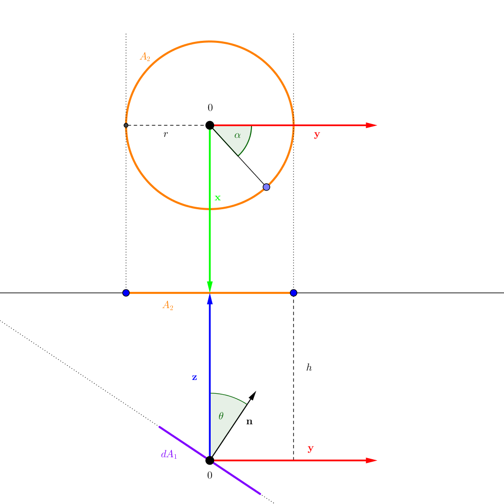
In this sketch, two views are included. Below the line in the middle is the \(yz\) plane. We are always free to choose a coordinate system best suited for our endeavour. Here we choose one, where our point is located in the origin. Its surface patch is oriented, such that its normal lies completely in the \(yz\) plane. The disk’s normal point along the negative \(z\) axis and is located directly on top of the point. As the surface patch already takes care of the orientation, the disk can be placed entirely in the \(xy\) plane, as shown in the top half of the image. The disk is located at \(z=h\) and has a radius \(r\). The angle between the differential area’s normal and the \(z\)-axis (or the disk’s negative normal) is \(\theta\). The parameter we will use to describe the points on the circle is \(\alpha\), the orientation as shown. For a more 3D-ish view of the scene, have a look at http://www.thermalradiation.net/sectionb/B-13.html. Our case here corresponds to the first case on the site. I will also use the same identifiers, so that we will arrive at the same expressions at the end.
With that in mind, we can define all relevant values. Let’s start with the directional cosines. Since our surface normal does not extend into the \(x\) direction, they have an angle of \(\pi /2\) (\(90^{\circ}\)) and therefore the cosine is \(0\). From the picture, we have the angle \(\theta\) between \(\mathbf{n}\) and \(z\), so that cosine is \(\cos \theta\). The last entry is between \(\mathbf{n}\) and \(y\). The angle beween them is \(\frac{\pi}{2} - \theta\). So we have \(\cos (\frac{\pi}{2} - \theta) = \sin \theta\).
\[\begin{aligned} l_1 &= \mathbf{n}\cdot\mathbf{x} = 0 \\ m_1 &= \mathbf{n}\cdot\mathbf{y} = \sin \theta \\ n_1 &= \mathbf{n}\cdot\mathbf{z} = \cos \theta \end{aligned}\]Next up are the values for the first surface (the differential area). Due to our choice of coordinate system, the point on the surface lies in the origin, so we have
\[\begin{aligned} x_1 &= 0\\ y_1 &= 0 \\ z_1 &= 0 \end{aligned}\]The last missing entries are the ones for the second area, or in this case, the area’s contour and the squared distance. First, the disk is located at a constant \(z\) value: \(h\). The disk’s contour is a circle, so the usual description for a circle can be used.
\[\begin{aligned} x_2 &= r \sin \alpha \\ y_2 &= r \cos \alpha \\ z_2 &= h \end{aligned}\]\(\alpha\) varies from \(0\) to \(2\pi\) for the whole circle. We could do only the half, since it’s symmetric, but it doesn’t matter much here. From that we can compute the differentials. For some function we have \(df = \frac{df}{dx} dx\), where \(\frac{df}{dx}\) is just the derivative with respect to \(dx\). Here, the parameter is \(\alpha\), so the result is:
\[\begin{aligned} dx_2 &= r \cos \alpha d\alpha\\ dy_2 &= -r \sin \alpha d\alpha \\ dz_2 &= 0 \end{aligned}\]The squared distance:
\[\begin{aligned} d^2 &= (r \sin \alpha-0)^2 + (r \cos \alpha)^2 + (h-0)^2 \\ &= r^2\sin^2\alpha + r^2\cos^2\alpha + h^2 \\ &= r^2(\sin^2\alpha + \cos^2\alpha) + h^2 \\ &= r^2 + h^2\end{aligned}\]We can now plug this into the equation from before. For better readability, I’ll do the terms one by one.
\[\begin{aligned} l_1\oint_C \frac{(z_2-z_1)dy_2 - (y_2-y_1)dz_2}{2\pi d^2} &= 0\oint_C \frac{(z_2-z_1)dy_2 - (y_2-y_1)dz_2}{2\pi r^2} \\ &= 0 \end{aligned}\] \[\begin{aligned}m_1\oint_C \frac{(x_2-x_1)dz_2 - (z_2-z_1)dx_2}{2\pi d^2} &= \frac{\sin \theta}{2\pi} \int_0^{2\pi} \frac{r\sin \alpha * 0 - hr\cos \alpha d\alpha}{r^2 + h^2 } \\ &= -\frac{hr\sin \theta}{2\pi(r^2+h^2)} \int_0^{2\pi} \cos \alpha d\alpha \\ &=-\frac{hr\sin \theta}{2\pi(r^2+h^2)} * 0 \\ &= 0\end{aligned}\] \[\begin{aligned} n_1\oint_C \frac{(y_2-y_1)dx_2 - (x_2-x_1)dy_2}{2\pi d^2} &= \frac{\cos \theta}{2\pi} \int_0^{2\pi} \frac{r\cos \alpha r\cos \alpha d\alpha - r\sin \alpha (-r\sin \alpha)d\alpha}{r^2 + h^2 } \\ &= \frac{\cos \theta}{2\pi(r^2+h^2)} \int_0^{2\pi} r^2\cos^2 \alpha + r^2\sin^2 \alpha d\alpha \\ &= \frac{r^2\cos \theta}{2\pi(r^2+h^2)} \int_0^{2\pi} \cos^2 \alpha + \sin^2 \alpha d\alpha \\ &= \frac{r^2\cos \theta}{2\pi(r^2+h^2)} \int_0^{2\pi} 1 d\alpha \\ &= \frac{r^2\cos \theta}{2\pi(r^2+h^2)} 2\pi \\ &= \frac{r^2}{r^2+h^2}\cos \theta\end{aligned}\]As this last one is the only not-null entry we finally have:
\[F_{dA_1,A_2} = \frac{r^2}{r^2+h^2}\cos \theta\]A slight bit of reformulation can be done. We introduce the variable \(H = \frac{h}{r}\). Then we can rearrange a part of the result:
\[\begin{aligned} \frac{r^2}{r^2+h^2} &= \frac{r^2}{r^2+h^2} *\frac{r^2}{r^2} \\ &= \frac{\frac{r^2}{r^2}}{\frac{r^2+h^2}{r^2}}\\ &= \frac{1}{1+ \frac{h^2}{r^2}} \\ &=\frac{1}{1 +H^2} \end{aligned}\]With that we get the final result in the same form as in the reference http://www.thermalradiation.net/sectionb/B-13.html:
\[F_{dA_1,A_2} = \frac{1}{1 +H^2}\cos \theta\]Next post we will incorporate the fact, that some parts of the disks may connect with our surface from behind. They have to be removed from the calculation, which complicates the whole thing a bit.