Geodesic Raytracer

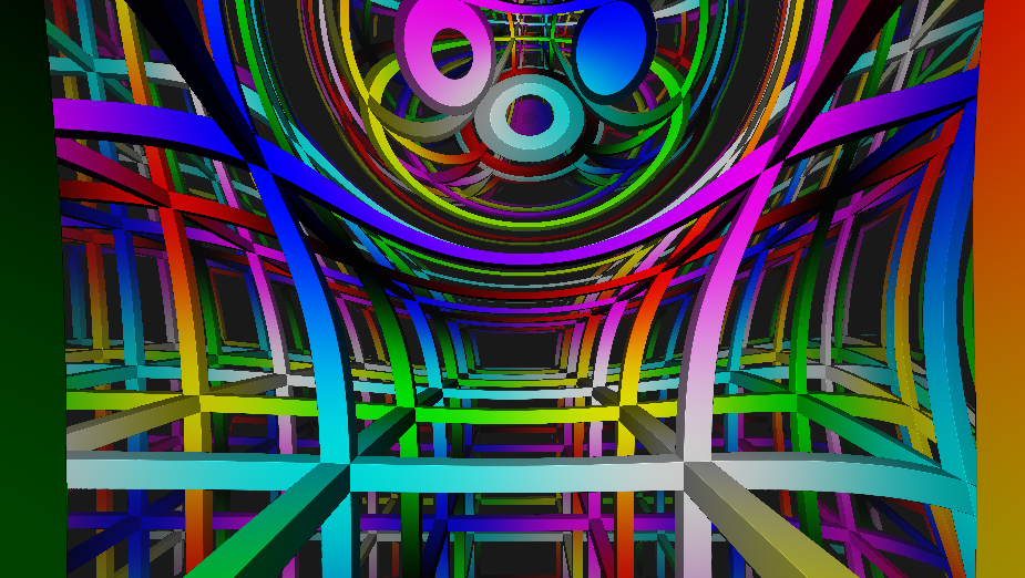
This is an example of a raytracer tracing rays through curved space, meaning some regions take longer for the ray to cross than others, despite looking "the same" in our normal 3D space. You can think of it similarly to gravitational effects bending space! A curve tracing out the locally shortest path through some space is called a geodesic. In uncurved space this is just a normal straight line.

The Shadertoy demo can be found here: https://www.shadertoy.com/view/fdBGDz

In our normal world, you can think about looking at a topographical map of some mountain range. Let's say you are just walking across a region (which we can say you are moving in 2D, your GPS coordinates basically) in some direction. And let's say you want to avoid getting too exhausted, so wherever you are you look in front of you (or your map) and basically go in the direction that takes the least amount of effort. So if you want to move in our 2D grid, you don't want to move up or down, as you would need to move the additional height. Think Pythagoras, the bottom smaller side will always be less than the hypothenuse spanned by the bottom and the height. In this case, the height at each point and our surroundings, which we could describe as a function $\operatorname{h}(x,y)$ would roughly tells us where to move next in order to minimize the effort. We call this measure of "how much does the terrain bend at a point" a metric, as it measures how much we need to adjust our units on the 2D map to incorporate height (I hope this simplification makes sense, please spare me, mathematicians!). The demo basically uses the same idea, but instead of a heightmap for each 2D ground point, we have a "height" for each point in space. The 2D heightmap needs an image with colors, a 3D object or something similar to show. Now for the 3D heightmap... well you could do some fancy tricks with 3D grids, where you pull together or push apart inner grid cells or use some transparency... but that is imho hard to understand. Or you could just display the graph in 4D! Well, that is kinda hard in our 3D world on the 2D screen. So I think the easiest way is to imagine the 2D heightmap analogy.

I was just trying to find some visualizations for this, but couldn't find a nice image (similarly to how I couldn't find the formulas used here, though I am sure I did at some point in the past!). I did find a nice video though! They don't just use heightmaps, but also some more general surfaces. Even visually explains more or less what happens in the shader later on, where it talks about moving locally step by step. The video can be seen here: https://youtu.be/NfqrCdAjiks.

So our stretching of space is given as a function $\operatorname{f}(x,y,z)$. This function can be defined in code and uses my simple GLSL library glsl-autodiff. The metric is then computed from the 4D graph (our heightmap) that this function describes. The shader performs a numerical integration of the ray according to local geodesics. The surface is defined as all points $\mathbf{r}$ of the following form:

$$\mathbf{r} = \begin{pmatrix} x\\ y\\ z\\ \operatorname{f}(x,y,z)\end{pmatrix}$$

This is the 4D point of the 3D heightmap. Similarly, when you leave out $z$ above, you have the formula for a point on a 2D heightmap in 3D space ($x,y$ describe your position on the map, the last $\operatorname{f}(x,y)$ is the height). And if you leave out $y$ as well, you get the point on the graph of a 1D function! So it's all the same idea!

In this case, the formulas can be simplified a bit compared to a more general hypersurface. This is done in code, as otherwise it would be too heavy to compute (even now, it might lag depending on your used GPU).

Here is a quick explanation of how we arrive at the formula used in the shader. It basically follows the above Wikipedia article and the one on Christoffel symbols. Personally, I can highly recommend the following playlist about tensor calculus and the corresponding book Introduction to Tensor Analysis and the Calculus of Moving Surfaces. This really helped me see both how cool it is to write stuff as tensors and in tensor notation and how much you can do with it.

First, let's define our (covariant) base vectors $\mathbf{e}_{i}, i = 1,2,3$. These define a coordinate system at each point. As we have a graph given by the above definition, we arrive at the base vectors as $\mathbf{e}_i = \frac{\partial \mathbf{r}}{\partial x_i}$, where we index $x,y,z$ in order so they become $x_1, x_2, x_3$. The partial derivatives here are geometrically just "move a bit along each parameter along the surface point to get a vector aligned to the surface". From graphics, you might know these as tangents and bitangents/binormals for a surface. For brevity, we will also write $\operatorname{f}_i = \frac{\partial \operatorname{f}}{\partial x_i}$ and $\operatorname{f}_{i,j} = \frac{\partial^2 \operatorname{f}}{\partial x_i \partial x_j}$

We then have:

$$\mathbf{e}_{1} = \begin{pmatrix} 1\\ 0\\ 0\\ \operatorname{f}_1\end{pmatrix}, \mathbf{e}_{2} = \begin{pmatrix} 0\\ 1\\ 0\\ \operatorname{f}_2\end{pmatrix}, \mathbf{e}_{2} = \begin{pmatrix} 0\\ 0\\ 1\\ \operatorname{f}_2\end{pmatrix}$$

The (covariant) metric tensor follows from this and basically defines, as the name says, a kind of metric on some space, which allows you to measure distances. The metric tensor can be indexed by two indices $g_{ij}$ and can be defined using the base vectors as:

$$g_{ij} = \mathbf{e}_i \cdot \mathbf{e}_j$$

So it measures the length and angles between the base vectors. It kinda makes sense then, that we use it to find the shortest path. Even if omitted in the notation, this may change for each point you evaluate it at. In the following, there will be a a bit of the Einstein summation convention. Simply said, diagonally aligned indices with the same name imply a summation, so $a^i b_i = a^1b_1 + a^2b_2 + a^3b_3$. As we are in 3D, the summation is from 1 to 3 (math convention, so we start at 1).

With that we have:

$$\begin{aligned} g_{ij} &= \mathbf{e}_i \cdot \mathbf{e}_j \\ &= \frac{\partial \operatorname{f}}{\partial x_i}\frac{\partial \operatorname{f}}{\partial x_j} \\ &= \operatorname{f}_i \operatorname{f}_j\\ g_{ii} &= \mathbf{e}_i \cdot \mathbf{e}_i \\ &= 1+ (\frac{\partial \operatorname{f}}{\partial x_i})^2\\ &= 1 + \operatorname{f}^2_i \end{aligned}$$

Written as a matrix this looks like the following:

$$g = \left[\begin{matrix}\operatorname{f}_{0}^{2} + 1 & \operatorname{f}_{0} \operatorname{f}_{1} & \operatorname{f}_{0} \operatorname{f}_{2}\\\operatorname{f}_{0} \operatorname{f}_{1} & f _{1}^{2} + 1 & \operatorname{f}_{1} \operatorname{f}_{2}\\\operatorname{f}_{0} \operatorname{f}_{2} & \operatorname{f}_{1} \operatorname{f}_{2} & \operatorname{f}_{2}^{2} + 1\end{matrix}\right]$$

Now, we will need to compute the inverse of that, which is also called the contravariant metric tensor $g^{ij}$ with the property $g^{ij} = g_{jk} = \delta^i_k$. This corresponds to inverting the matrix above. You can do it by hand, I used a symbolic math library, as it is a lot to write... This results in:

$$\begin{aligned} g^{-1} = \left[\begin{matrix}\frac{\operatorname{f}_{1}^{2} + \operatorname{f}_{2}^{2} + 1}{\operatorname{f}_{0}^{2} + \operatorname{f}_{1}^{2} + f _{2}^{2} + 1} & - \frac{\operatorname{f}_{0} \operatorname{f}_{1}}{\operatorname{f}_{0}^{2} + \operatorname{f}_{1}^{2} + \operatorname{f}_{2}^{2} + 1} & - \frac{\operatorname{f}_{0} \operatorname{f}_{2}}{\operatorname{f}_{0}^{2} + \operatorname{f}_{1}^{2} + \operatorname{f}_{2}^{2} + 1}\\- \frac{\operatorname{f}_{0} \operatorname{f}_{ 1}}{\operatorname{f}_{0}^{2} + \operatorname{f}_{1}^{2} + \operatorname{f}_{2}^{2} + 1} & \frac{\operatorname{f}_{0}^{2} + \operatorname{f}_{2}^{2} + 1}{ \operatorname{f}_{0}^{2} + \operatorname{f}_{1}^{2} + \operatorname{f}_{2}^{2} + 1} & - \frac{\operatorname{f}_{1} \operatorname{f}_{2}}{\operatorname{f}_{0}^{2} + \operatorname{f}_{1 }^{2} + \operatorname{f}_{2}^{2} + 1}\\- \frac{\operatorname{f}_{0} \operatorname{f}_{2}}{\operatorname{f}_{0}^{2} + \operatorname{f}_{1}^{2} + \operatorname{f}_{2}^{2} + 1} & - \frac{\operatorname{f}_{1} \operatorname{f}_{2}}{\operatorname{f}_{0}^{2} + \operatorname{f}_{1}^{2} + \operatorname{f}_{2}^{2} + 1} & \frac{\operatorname{f}_ {0}^{2} + \operatorname{f}_{1}^{2} + 1}{\operatorname{f}_{0}^{2} + \operatorname{f}_{1}^{2} + \operatorname{f}_{2}^{2} + 1}\end{matrix}\right] \end{aligned}$$

Here we can see $\operatorname{f}_{0}^{2} + \operatorname{f}_{1}^{2} + \operatorname{f}_{2}^{2} = ||\nabla\operatorname{f}||^2$ quite often.

The dual basis, also called the contravariant base vectors are then defined by "raising the indices":

$$\mathbf{e}^i = g^{ij}\mathbf{e}_{j}$$

As an example, here is the result of that operation for $\mathbf{e}^0$, the others look very similar.

$$\begin{aligned} \mathbf{e}^0 &= \left[\begin{matrix}\frac{\operatorname{f}_{1}^{2} + \operatorname{f}_{2}^{2} + 1}{\operatorname{f}_{0}^{2} + \operatorname{f}_{1}^{2} + f _{2}^{2} + 1}\\- \frac{\operatorname{f}_{0} \operatorname{f}_{1}}{\operatorname{f}_{0}^{2} + \operatorname{f}_{1}^{2} + \operatorname{f}_{2}^{2} + 1}\\- \frac{\operatorname{f}_{0} \operatorname{f}_{2}}{\operatorname{f}_{0}^{2} + \operatorname{f}_{1}^{2} + \operatorname{f}_{2}^{2} + 1}\\\frac{\operatorname{f}_{0}}{\operatorname{f}_{0}^ {2} + \operatorname{f}_{1}^{2} + \operatorname{f}_{2}^{2} + 1}\end{matrix}\right]\\ &= \frac{1}{\operatorname{f}_{0}^{2} + \operatorname{f}_{1}^{2} + f _{2}^{2} + 1} \left[\begin{matrix}\operatorname{f}_{1}^{2} + \operatorname{f}_{2}^{2} + 1\\- \operatorname{f}_{0} \operatorname{f}_{1}\\- \operatorname{f}_{0} \operatorname{f}_{2}\\\operatorname{f}_{0}\end{matrix}\right] \\ &= \frac{1}{1+||\nabla\operatorname{f}||^2 } \left[\begin{matrix}\operatorname{f}_{1}^{2} + \operatorname{f}_{2}^{2} + 1\\- \operatorname{f}_{0} \operatorname{f}_{1}\\- \operatorname{f}_{0} \operatorname{f}_{2}\\\operatorname{f}_{0}\end{matrix}\right] \end{aligned}$$

This is used to define the so called Christoffel symbols:

$$\Gamma^k_{ij} = \frac{\partial \mathbf{e}_j}{\partial x_i} \cdot \mathbf{e}^k$$

These are a bit harder to conceptualize, but they measure a kind of change along the surface.

Importantly, we have to derive $\mathbf{e}_j$ again. As the first 3 entries of $\mathbf{e}_j$ are constants, they will become $0$, so the dot product will also just be the last coordinate times the last entry of $\mathbf{e}^k$.

$$\begin{aligned} \frac{\partial \mathbf{e}_j}{\partial x_i} &= \begin{pmatrix}0 \\ 0 \\ 0 \\ \frac{\partial \operatorname{f}_j}{\partial x_i} \end{pmatrix} &= \begin{pmatrix}0 \\ 0 \\ 0 \\ \ \operatorname{f}_{j,i} \end{pmatrix} \end{aligned}$$

It should be noted, that we are generally dealing and defining functions that are smooth, so the mixed partial derivatives will be symmetrically equal $\operatorname{f}_{j,i} = \operatorname{f}_{i,j}$.

The last coordinate of the contravariant bases $\mathbf{e}^k$ (see above) has the nice form $\frac{\operatorname{f}_{k}}{\operatorname{f}_{0}^ {2} + \operatorname{f}_{1}^{2} + \operatorname{f}_{2}^{2} + 1} = \frac{\operatorname{f}_{k}}{1 + ||\nabla\operatorname{f}||^2}$.

So the overall expression for the Christoffel symbols is:

$$\Gamma^k_{ij} = \frac{\operatorname{f}_{j,i} \operatorname{f}_{k}}{1+ ||\nabla\operatorname{f}||^2}$$

The geodesics of a curve $\gamma(t)$ (the ray we want to trace, which might bend due to the metric) can be described using the geodesic equation:

$$\frac{d^2 c^k}{dt^2} + \Gamma_{ij}^k \frac{dc^i}{dt}\frac{dc^k}{dt} = 0$$

We can directly solve for the acceleration:

$$\frac{d^2 c^k}{dt^2} = - \Gamma_{ij}^k \frac{dc^i}{dt}\frac{dc^k}{dt}$$

We can use the ray's current velocity ($\frac{d\mathbf{c}}{dt}$) as initial values in the above equation to compute the acceleration and from that the new velocity and position.