Curvature Visualization of Implicit Surfaces

The following shows two types of curvature visualizations computed live from the implicit surface definition. Curvature, as the name suggests, measures how much a curve or surface "curves", meaning diverges from a straight line/plane. You can find a general overview on Wikipedia.

As Shadertoy embeds don't seem to work anymore, here are screenshots and links to the shaders.

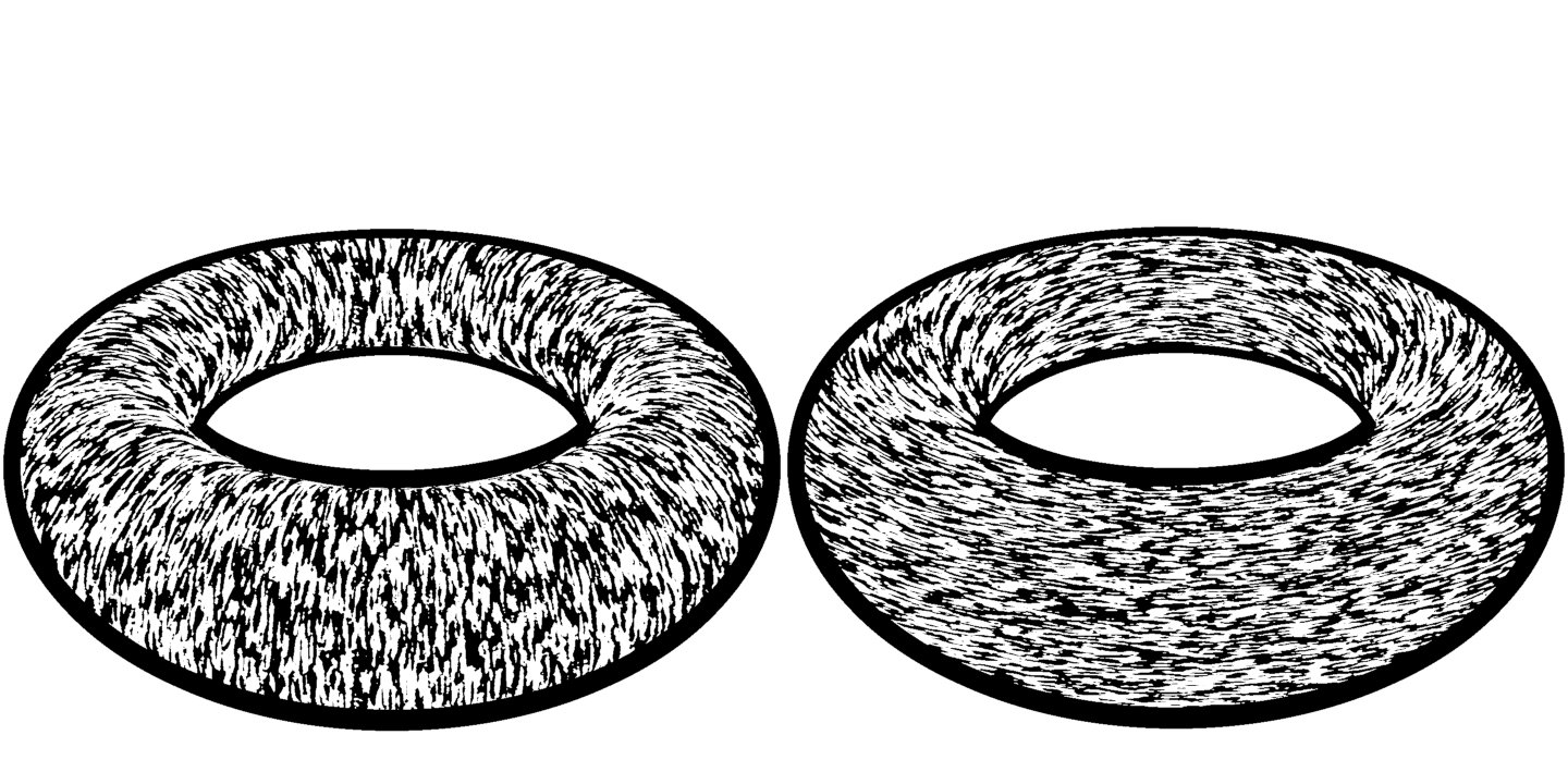
You can find the first shader here: https://www.shadertoy.com/view/4stSRf

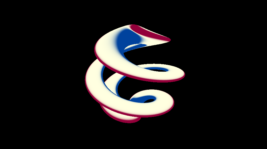
In the second example, the Gaussian curvature is computed from the Hessian and gradient.

You can find the second shader here: https://www.shadertoy.com/view/Nd3GRS

The shaders use my automatic differentiation pack for GLSL (https://github.com/sibaku/glsl-autodiff). Basically, this computes derivatives of expressions by wrapping each operation and adding a bit of additional data to each number. The nice thing is, that it is exact minus numerical precision without too much overhead. This is in stark contrast to numerical differentiation, but requires implementing all operations using custom types (much easier in languages with operator overloading).

The first example utilizes a special property of distance fields, where the Hessian matrix is the Shape operator. I won't go into all the details here, but it basically follows from the following: You can get the normal of an implicit surfaces, which distance fields are, by calculating its gradient. Since the gradient points into the direction of largest increase, it will be perpendicular to the surface, as the surface is given as all points for which the implicit function has a specific constant value, usually 0, so the value does not change along the surface, but changes the most if you move straight away from it. For distance fields, the gradient is normalized as well. This also makes sense, because it measures the rate of change. If you move straight away from the surface, your distance to it will also increase by that same amount and that is the value that a distance field measures. In differential geometry, you can define the so called Shape operator as the derivative of the normal field (the function assigning a unit normal to each point). As this is exactly the distance field gradient, its Hessian is the Shape operator. This operator has a few nice properties which are also listed on the Wikipedia article linked above. Here, we use one of those:

Its two non-zero eigenvalues correspond to the principal curvatures (largest and leas curvature) and the corresponding eigenvectors are the directions. One of the eigenvalues is zero, as the normal defines the null-space of the Shape operator. This is used in the first shader. For that, the shader uses a simple iterative algorithm called Jacobi Iteration. The curvature directions are then projected onto the screen, so we get a 2D direction. This is then used in the final step to actually display the directions using a simple version of Line integral convolution. It basically steps along a the direction in a random noise texture and accumulates values along the way. As the directions are aligned to the surface, this results in stroke like lines. Due to the random texture, these lines don't have common aliasing or spacing issues, but aren't overly regular, so they have a more painterly look instead of a nice and clean "math" look.

For the second shader, we compute an implicit surface's Gaussian curvature. For distance fields, this would be a bit easier, as the Gaussian curvature is given by the determinant of the hessian. In this shader, we use the general formula for implicit surfaces given here. The nice thing about this value is that it is an "intrinsic" value of the surface, so it is independent of the surrounding space. The second shader colorizes the value of the Gaussian curvature at each point, blue for negative curvature, red for positive, and white for no curvature.