Pixel Collisions

A small conversation on Bluesky made me think about the following issue: Given a collision shape represented as pixels, how can we get the necessary information to handle collisions. Mainly this means: How to generate normals for each pixel, as the normal and position are generally the geometric information you will use in any kind of collision system.

The simplest (but also slightly complex) solution is the following: Each pixel is a small square taking up space in your world. A square has 4 sides with 4 pretty simple normals: They just point in the positive or negative x and y directions. We then need to determine which side we are intersecting/closest to and use that normal. This determination might be a bit cumbersome. Additionally, we will run into a larger issue: The pixels might represent a non-horizontal, non-vertical curved shape. But this solutions only gives us horizontal and vertical normals. This makes handling slopes and other curved collision objects really annoying.

This article will show you a way to create normals for each pixel in a collision shape which follow the shape of the shape boundary. These can then be used as you see fit in your use case. Below is a basic demo implementing this method and combines it with a very basic physics simulation of some balls being dropped from above and bouncing on the obstacles. You can draw the obstacles yourself with your mouse. Just click and drag . There are some options and shortcuts to operate the demo. You can have a look at the full, commented source code HERE. It is (hopefully) kept simple to make it clear how everything works. You might also encounter some bugs in the physics, have fun!

Below the demo, I will explain how this works and also a few things to be careful about.

Explanation

We won't go into a full theoretical background, but I will try to give you a basic idea of how this works and provide you with a few pointers to the math that is behind it. At the end, I will also mention some additional things that can be used to augment this.

First, let us define the data we are working with. We will use a binary grid/image to represent our obstacle. Let's use 1 equals free space, and 0 equals obstacles for this explanation. This is just a convention, there isn't too much that changes if you do it the other way around. The demo actually uses the other way, because it makes computing values along the border of the grid a bit nicer. You just need to be aware of what you use! Let's also say, we can access a value of the grid at position $(x,y)$ as $\operatorname{f}(x,y)$. Depending on your programming language, this might be implemented as a 1D or 2D array, looking like one of the following:

// language has a native 2D array
f[x,y]

// language uses nested arrays (each array element is an array)
f[x][y] // another convention is f[y][x]

// language or user preference only uses 1D array (the demo does this)
f[x + y*width] // width is the width of the grid

// 2D indices can be converted to 1D using the above formula

This setup allows us to easily check, whether a collision occurs at a pixel by just checking if it is 0 or 1 in the grid! While you can of course do all kind of other fancy things, this is what we will be working with as far as detection goes. For now, we will also assume that you won't move more than one pixel in a frame, so you can't "skip" pixels. In the extensions sections, I will show you a way to relax this condition. In general, this is probably not too much of an issue, as you can alleviate it with checking inbetween-positions or raycasts.

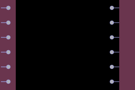
Let us first imagine a view of a wall and only concern ourselves with the x direction. This wall has a left and right side, but for now, we will only look at the right half.

Here is what it looks like, with the wall colored in black, the free space in reddish.

On the right side of the right half we have free space and on the left side there are obstacles. We are interested in normals at the pixels at the boundary, as this is where collisions happen. We will say, that the boundary pixels are those which are adjacent to free pixels.

We start with specifying what we want the normal to be: It should point right at the boundary, meaning that the x coordinate should be 1. How can we do that?

We can observe, that the values of the grid change at the boundary. So how about the following idea: At a position $(x,y)$, compute the following value: $\operatorname{f}(x+1,y) - \operatorname{f}(x,y)$.

Since we are at the boundary (which is part of the obstacle), $\operatorname{f}(x,y)$ will be $0$ and one to the right is free space, so $\operatorname{f}(x+1,y)$ will be $1$!, meaning $\operatorname{f}(x+1,y) - \operatorname{f}(x,y) = 1- 0 = 1$. This is exactly what we want!

What happens at other points away from the boundary? Well, there both the left and right side will have the same value and the expression is $0$. This makes sense, as we don't really have a boundary in a region without change. There is an exception to that though. While we did not yet consider it, what happens on the left border of the wall in the left half? Does our formula hold up?

Well, sadly, it doesn't work as it should, because the pixel to the right is also part of the boundary! So the expression above evaluates to $0$. And if we look at the free pixels directly next to the wall, there will be a normal outside the boundary... not really what we wanted, but doesn't break anything and it might make you hopeful that we are on the right track, as the normal points away from the left boundary.

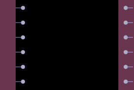
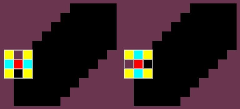
The result looks like the following, with normals visualized as small lines with a circle at the pixel center.

But what if we just looked to the left instead? Then we should also switch around the order to get a normal pointing left ($x=-1$).

So we have $\operatorname{f}(x,y) - \operatorname{f}(x-1,y) = 0 - 1 = -1$, which is correct. This will similarly not work though with the previous wall side and also result in $0$ in all non-boundary pixels aside from the free spaces directly next to the right boundary.

But how about the following idea: Just combine both values! We have established, that the first version will only result in 1 in boundaries on the right (not on the left, where it is actually 0!) and the second version will only evaluate to -1 on boundaries on the left (not on the right, again 0!). Otherwise they are zero. So they don't interfere with each other, meaning we can add them together:

$$\begin{aligned} &\operatorname{f}(x+1,y) - \operatorname{f}(x,y) + \operatorname{f}(x,y) - \operatorname{f}(x-1,y) \\ &= \operatorname{f}(x+1,y) - \operatorname{f}(x-1,y) \\ &= \Delta_{x}(x,y) \end{aligned}$$

We use $\Delta_{x}(x,y)$ ("Delta x at $(x,y)$") as a name for this quantity. This delta symbol is often used for a difference of sorts.

You can verify yourself that this yields the results of the previous two paragraphs combined! You can also observe that this also creates a normal at the free spaces adjacent to your boundary, which might be handy! For example, you could use surrounding normals for smoothing.

NOTE You might notice one important thing: This requires the obstacle object to be at least two pixels wide! This also makes sense though. If you look not too closely at a needle or string, you basically just see a line. A line has no "surface" and thus you can't determine a surface direction. Same with single pixel lines, they don't give us enough information for a normal, as the represent a boundary to both a left and right side. So you will need to make sure to draw your obstacles with at least two pixels, otherwise there might be issues, which you can try to observe in the demo!

The result now looks like this!

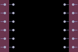
The exact same discussion as before can be done with a floor/ceiling, so a wall in the y direction. For that direction we then get accordingly:

$$\begin{aligned} &\operatorname{f}(x,y+1) - \operatorname{f}(x,y-1) \\ &= \Delta_{y}(x,y) \end{aligned}$$

Now here is the pretty incredible part: When you put these two values together into a vector, you get the normal of the boundary, not just for these perfectly aligned walls, but also for curved surfaces! You can think about this as follows: Since we are in 2D, we have two base directions with which we can create any vector (the x,y coordinates with their corresponding axis vector!). Similarly, we just found the expressions for the two "base" walls, horizontal and vertical. All other walls will just be a kind of combination between these two main wall types.

Of course, with just 4 points to evaluate and a binary grid, the combinations/slopes this can represent are limited, but it already works! Let us call this vector (for reasons) $\mathbf{g}(x,y)$:

$$\begin{aligned} \mathbf{g}(x,y) &= \begin{pmatrix}\operatorname{f}(x+1,y) - \operatorname{f}(x-1,y) \\ \operatorname{f}(x,y+1) - \operatorname{f}(x,y-1) \end{pmatrix} \\ &= \begin{pmatrix}\Delta_{x}(x,y) \\ \Delta_{y}(x,y)\end{pmatrix} \end{aligned}$$

The length of this vector gives us some information about how much the values change in each direction. If its length is not zero (which it won't be at a boundary), we can also normalize it, to get the final collision normal $\mathbf{n}(x,y)$. When coding, you would need to check, if the length is not zero, before normalization.

$$\begin{aligned} \mathbf{n}(x,y) &= \frac{\mathbf{g}(x,y)}{||\mathbf{g}(x,y)||} \\ &= \begin{pmatrix}n_x \\ n_y\end{pmatrix} \end{aligned}$$

$||\cdot||$ means: Length of the vector inside the brackets.

You can also retrieve the angle $\alpha$ ("alpha") via the components of the normal as $\alpha = \arctan (\frac{n_y}{n_x})$. Using the arc tangent function requires taking care of signs, so most languages already have a built-in function for that:

$$\alpha = \operatorname{atan2}(n_y,n_x)$$

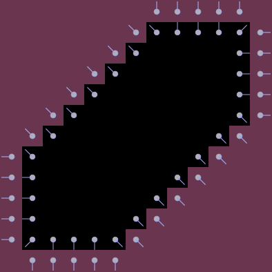
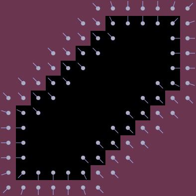
The result for a more complex shape looks like the following. You can see that the normals along the diagonal looks like you would expect them to look for a diagonal! Even if the pixel structure is just a stair shape.

One additional thing we can do to make this cover a few more types of "slopes" is to also look at the surroundings. For example, for $(x,y)$ let us also look at $\Delta_{x}(x,y+1)$ and $\Delta_{x}(x,y-1)$ for the x direction and $\Delta_{y}(x+1,y)$ and $\Delta_{y}(x-1,y)$ for the y direction.

Of course, as these values are a bit further away from $(x,y)$, we don't want them to be as important as $\Delta_{x}(x,y)$ and $\Delta_{y}(x,y)$, the original entries of our vector $\mathbf{g}$.

We can express this by weighing the results. We will weight the two left/right and up/down groups the same as to not prefer a direction, which leaves us with two groups: The center group, which is the original function and the offsets. Here highlighted is the x direction on the left and the y direction on the right. The middle weight is highlighted in a blueish color, while yellow signals the outer groups:

You can of course define your own weights, but we will show two common ones.

$$\begin{aligned} \operatorname{Sobel}_x(x,y) &= \Delta_{x}(x,y+1) + 2\Delta_{x}(x,y) + \Delta_{x}(x,y-1)\\ \operatorname{Sobel}_y(x,y) &= \Delta_{y}(x+1,y) + 2\Delta_{y}(x,y) + \Delta_{y}(x-1,y) \end{aligned}$$

and

$$\begin{aligned} \operatorname{Scharr}_x(x,y) &= 47\Delta_{x}(x,y+1) + 162\Delta_{x}(x,y) + 47\Delta_{x}(x,y-1)\\ \operatorname{Scharr}_y(x,y) &= 47\Delta_{y}(x+1,y) + 162\Delta_{y}(x,y) + 47\Delta_{y}(x-1,y) \end{aligned}$$

You can use these x,y function pairs as entries of $\mathbf{g}$. So for example:

$$\mathbf{g}_{\text{Sobel}} = \begin{pmatrix}\operatorname{Sobel}_x(x,y)\\ \operatorname{Sobel}_y(x,y)\end{pmatrix}$$

The Sobel operator results in this:

You can see that more pixels around the shape get normals and that it better adjusts to shape changes, for example on the left corner, where the diagonal ends.

Since we normalize the normal vector anyways, we don't need to care much about the weights increasing the values. All of these methods are implemented in the demo and you can check their differences but also observe that they generate fitting normals for oriented and curved boundaries (as much as that means with pixels...) without any issues. With this, you can generate normals for your pixel based collision shapes!

One final note about boundaries of the grid. Our functions look left, right, top and bottom of our position. This might lie outside the grid. There are multiple ways to handle this, such as mirroring, repeating and others. In the demo, I used the simple variant of ignoring outside values, basically setting all outside values to 0. Since 0 means obstacle in the above derivations, this will result in normals being generated at free boundary pixels. This isn't an issues, as they are on free space so aren't used, but I thought they are distracting in the demo. That's why the demo uses 1 for obstacles and 0 for free pixels. The only change in the formulas is, that we will need to reverse the result of $\mathbf{g}$/Sobel/Sharr/..., meaning negate each entry. So a very simple change!

FINISH

Below will be some additional notes, short mathematical explanations and then some additions that can improve on this. Hopefully, the above explanations already helped you understanding why this works, the details are just a bit more general.

You might be wondering about the names I gave to the functions above, "Sobel" and "Sharr". If you have done any image processing before, this whole section might have sounded familiar. Evaluating pixels around a central pixel and weighing them together is just what a filter in image processing does! And two examples for an edge-detection filter are the Sobel and the Sharr filter! You can read about it here. You might even have used at least one of them before in an image editing tool!

Mathematical Background

We won't do a full derivation of anything here, but I just want to give you some basic idea of what this all means in maybe more familiar terms. You are free to skip to the final extension section if you are not interested in the maths.

First of all, let us look at the expression $\operatorname{f}(x+1,y) - \operatorname{f}(x,y)$.

We can also write this as $\frac{\operatorname{f}(x+1,y) - \operatorname{f}(x,y)}{1}$. It might be more familiar, if we replace the $1$ with some generic value $h$:

$$\frac{\operatorname{f}(x+h,y) - \operatorname{f}(x,y)}{h}$$

If you have not taken higher math classes, one additional simplification might make it clearer. Above, $y$ does not change, so let's for a moment pretend this function has only one variable $x$:

$$\frac{\operatorname{f}(x+h) - \operatorname{f}(x)}{h}$$

You might recognize this as a difference quotient! If we were to pretend that our values weren't on a grid, but instead a continuous function, then in the limit of $h\rightarrow 0$ this will yield the derivative!

$$\lim_{h\rightarrow 0}\frac{\operatorname{f}(x+h) - \operatorname{f}(x)}{h} = \operatorname{f}'(x)$$

Our special form with putting left and right together is called the central difference and has some of its own special properties, which we won't get into here. But for simplicity, this is also just an expression for the derivative.

The 2D version of this derivative also has a name: Partial derivative. It measures the rate of change of a function along one of the variables it depends on! You might know the notation $\operatorname{f}'(x) = \frac{d\operatorname{f}(x)}{dx}$. For partial derivatives, the "d" is replaced by the symbol $\partial$, to make a distinction.

$$\lim_{h\rightarrow 0}\frac{\operatorname{f}(x+h,y) - \operatorname{f}(x,y)}{h} = \frac{\partial \operatorname{f}(x,y)}{\partial x}$$

And similarly for $y$: $\frac{\partial \operatorname{f}(x,y)}{\partial y}$

You can read the $\partial$ as "d" or "del", if you want to make it clear.

The vector consisting of all partial derivatives of a function is called its gradient, written as $\nabla \operatorname{f}(x,y)$ or $\operatorname{grad} \operatorname{f}(x,y)$. You can in this case pronounce $\nabla$ as "grad" or "gradient". This is why we named the vector above $\mathbf{g}$, for gradient. Be careful though, because this so called "nabla" operator is used in quite a few ways, so don't take this as the last word.

$$\nabla \operatorname{f}(x,y) = \begin{pmatrix}\frac{\partial \operatorname{f}(x,y)}{\partial x} \\ \frac{\partial \operatorname{f}(x,y)}{\partial y} \end{pmatrix}$$

The gradient has the amazing property that it always points into the direction of greatest increase. So first off, if your obstacle object has values smaller than the outside values, this means that the gradient will point outside of the object! Just what we need! As we assumed for this, that the object is actually given as a continuous function, we might define the object or boundary (there is a distinction which relates to differentiability, but that is also another topic) as all points that have a certain value. In our binary case, we said that all points with a value of 0 are part of the obstacle object! This is a case of a so called "implicit surface", where we can recover the normal at any point via its gradient! Also works in 3D! This is also related to the extensions.

This was the very quick and dirty mathematical background of what we have done above. If you want to learn more about any of these, there are many resources if you just type on some of the keywords.

Extensions

There are many things you could do, from special handling for lines, to smoothing the resulting normal vectors or doing some other averaging scheme. Here, I want to highlight three extensions that I think could be useful.

First: Add gray values to the grid. The function we defined above does not require zeros and ones, it can also take in grayscale. So if you use some aliasing when drawing the shapes or maybe add a bit of blur, this might smooth out the normals a bit more around non horizontal or vertical segments.

Second: Morphoplogy operations. This might sound like a complicated word, but it isn't very hard. It is similar to a normal filter! A general overview can be found at Wikipedia. Basically, operations such as erosion or dilation allow us to close small holes or remove small noisy parts. There are others as well. This might be useful, if you have a very complex shape, but want to automatically make it a bit more cohesive for collisions.

Third: The most complicated of these three extensions. I mentioned in the beginning, that objects should not move more than one pixel per frame/step. The reason is that you could move through an obstacle pixel into a shape, where no normals exist anymore, thus preventing further collisions as well. One solution is to utilize (signed) distance fields. There are many ways to do this, but here is the basic idea. For each pixel, search for the closest boundary pixel (a pixel which has a free pixel next to it) and record the distance to it. For a signed distance field, which is preferable, you can also add a negative sign to the distance inside of a shape. This could even be done brute force, though that would be very slow. A fast and easy to implement algorithm is for example the Meijster distance transform, but there are others as well.

Now, a distance field is a type of implicit surface, as mentioned in the mathematical background. If you calculate the gradient (you can even use our method on the distance values!), you get a normal for each point in and outside of the shape (there are a few here negligible exceptions). If the field is signed, they will even be correctly oriented! Not only that, the gradient (multiplied by the negative signed distance) is the translation vector to the boundary!

With that, you can check for every point if it's inside the shape (either just the binary values or the signed distance) and you can move a point to the nearest surface. So, as long as you don't completely move through a full object in a frame, you can recover intersections with the collisions of multiple pixels with this technique!