View-factor disk with oriented area element

View-factor fully visible

One method for computing diffuse global illumination is radiosity (Radiosity). The solution to the illumination problem is gained by bouncing light around all the surfaces in a scene until nothing changes anymore. To do this, one has to consider how much of the light arriving at one surface will be sent to another one. The proportion of the total light exchange is called view factor (sometimes form factor or configuration factor).

I once had to deal with a related problem, not radiosity, where I had to more or less compute the view factor of a differential surface patch (a point on a surface) and a disk. The point is located along the disk's normal, but rotated somewhat. This post will deal with the case, that disk is fully visible. You can find this and many other formulas at http://www.thermalradiation.net/, even with references on where they are from. Sadly, when I looked up the sources for the specific formulas, they were horribly described and nearly unreadable imho. So I plan to do a (hopefully) more easily understood derivation.

The quantity we want to compute is as follows:

$$F_{dA_1,A_2} = \int_{A_2}\frac{\cos\beta_1 \cos\beta_2 dA_2}{\pi r^2}$$

We have a differential area $dA_1$ and an area $A_2$. We now integrate over $A_2$, and for every differential area $dA_2$ on it, we connect it to $dA_1$. The length of that connection is $r$, the angle with the normal of $dA_1$ is $\cos\beta_1$ and the angle with the normal of $dA_2$ is $\cos\beta_2$. There are various ways to deal with that problem depending on the geometry involved. One way can be found in a paper by Sparrow ("A new and Simpler Formulation for Radiative Angle Factors",1963). The key insight is, that Stoke's theorem can be used to compute that area integral, meaning you can transform the integral over the area into one over the surface's contour. The result is the following:

$$\begin{aligned} F_{dA_1,A_2} &= l_1\oint_C \frac{(z_2-z_1)dy_2 - (y_2-y_1)dz_2}{2\pi d^2} \\&+ m_1\oint_C \frac{(x_2-x_1)dz_2 - (z_2-z_1)dx_2}{2\pi d^2} \\ &+ n_1\oint_C \frac{(y_2-y_1)dx_2 - (x_2-x_1)dy_2}{2\pi d^2} \end{aligned}$$

$l_1, m_1, n_1$ are the components of $dA_1$'s normal expressed in a given coordinate system with the $\mathbf{x}, \mathbf{y}, \mathbf{z}$ axes. Or, as worded in the paper, they are the directional cosines, the cosines of the angle between the normal and each axis (or in other words, their dot product). The $\oint_C$ notation means, that we need a closed boundary curve, meaning we end where we start. The other values are the coordinates, their index representing which surface they belong to. Since we only go over the surface $A_2$, only those coordinates vary. $d^2$ is the squared distance between two points, so it can be computed as:

$$d^2 = (x_2 - x_1)^2 + (y_2 - y_1)^2 + (z_2 - z_1)^2$$

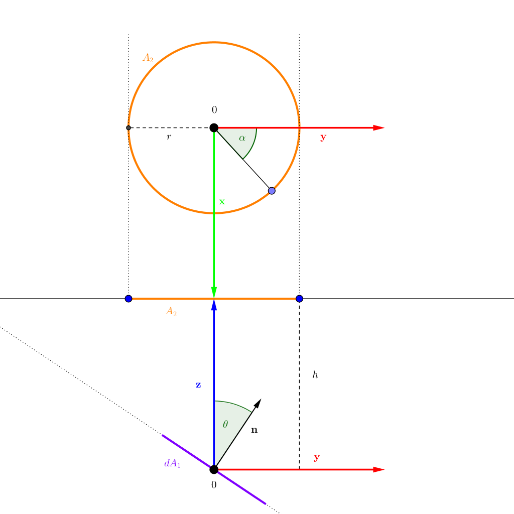
We can now get to our problem. First, let's sketch the setup:

In this sketch, two views are included. Below the line in the middle is the $yz$ plane. We are always free to choose a coordinate system best suited for our endeavor. Here we choose one, where our point is located in the origin. Its surface patch is oriented, such that its normal lies completely in the $yz$ plane. The disk's normal point along the negative $z$ axis and is located directly on top of the point. As the surface patch already takes care of the orientation, the disk can be placed entirely in the $xy$ plane, as shown in the top half of the image. The disk is located at $z=h$ and has a radius $r$. The angle between the differential area's normal and the $z$-axis (or the disk's negative normal) is $\theta$. The parameter we will use to describe the points on the circle is $\alpha$, the orientation as shown. For a more 3D-ish view of the scene, have a look at http://www.thermalradiation.net/sectionb/B-13.html. Our case here corresponds to the first case on the site. I will also use the same identifiers, so that we will arrive at the same expressions at the end.

With that in mind, we can define all relevant values. Let's start with the directional cosines. Since our surface normal does not extend into the $x$ direction, they have an angle of $\pi /2$ ($90^{\circ}$) and therefore the cosine is $0$. From the picture, we have the angle $\theta$ between $\mathbf{n}$ and $z$, so that cosine is $\cos \theta$. The last entry is between $\mathbf{n}$ and $y$. The angle beween them is $\frac{\pi}{2} - \theta$. So we have $\cos (\frac{\pi}{2} - \theta) = \sin \theta$.

$$\begin{aligned} l_1 &= \mathbf{n}\cdot\mathbf{x} = 0 \\ m_1 &= \mathbf{n}\cdot\mathbf{y} = \sin \theta \\ n_1 &= \mathbf{n}\cdot\mathbf{z} = \cos \theta \end{aligned}$$

Next up are the values for the first surface (the differential area). Due to our choice of coordinate system, the point on the surface lies in the origin, so we have

$$\begin{aligned} x_1 &= 0\\ y_1 &= 0 \\ z_1 &= 0 \end{aligned}$$

The last missing entries are the ones for the second area, or in this case, the area's contour and the squared distance. First, the disk is located at a constant $z$ value: $h$. The disk's contour is a circle, so the usual description for a circle can be used.

$$\begin{aligned} x_2 &= r \sin \alpha \\ y_2 &= r \cos \alpha \\ z_2 &= h \end{aligned}$$

$\alpha$ varies from $0$ to $2\pi$ for the whole circle. We could do only the half, since it's symmetric, but it doesn't matter much here. From that we can compute the differentials. For some function we have $df = \frac{df}{dx} dx$, where $\frac{df}{dx}$ is just the derivative with respect to $dx$. Here, the parameter is $\alpha$, so the result is:

$$\begin{aligned} dx_2 &= r \cos \alpha d\alpha\\ dy_2 &= -r \sin \alpha d\alpha \\ dz_2 &= 0 \end{aligned}$$

The squared distance:

$$\begin{aligned} d^2 &= (r \sin \alpha-0)^2 + (r \cos \alpha)^2 + (h-0)^2 \\ &= r^2\sin^2\alpha + r^2\cos^2\alpha + h^2 \\ &= r^2(\sin^2\alpha + \cos^2\alpha) + h^2 \\ &= r^2 + h^2\end{aligned}$$

We can now plug this into the equation from before. For better readability, I'll do the terms one by one.

$$\begin{aligned} l_1\oint_C \frac{(z_2-z_1)dy_2 - (y_2-y_1)dz_2}{2\pi d^2} &= 0\oint_C \frac{(z_2-z_1)dy_2 - (y_2-y_1)dz_2}{2\pi r^2} \\ &= 0 \end{aligned}$$

$$\begin{aligned}m_1\oint_C \frac{(x_2-x_1)dz_2 - (z_2-z_1)dx_2}{2\pi d^2} &= \frac{\sin \theta}{2\pi} \int_0^{2\pi} \frac{r\sin \alpha * 0 - hr\cos \alpha d\alpha}{r^2 + h^2 } \\ &= -\frac{hr\sin \theta}{2\pi(r^2+h^2)} \int_0^{2\pi} \cos \alpha d\alpha \\ &=-\frac{hr\sin \theta}{2\pi(r^2+h^2)} * 0 \\ &= 0\end{aligned}$$

$$\begin{aligned} n_1\oint_C \frac{(y_2-y_1)dx_2 - (x_2-x_1)dy_2}{2\pi d^2} &= \frac{\cos \theta}{2\pi} \int_0^{2\pi} \frac{r\cos \alpha r\cos \alpha d\alpha - r\sin \alpha (-r\sin \alpha)d\alpha}{r^2 + h^2 } \\ &= \frac{\cos \theta}{2\pi(r^2+h^2)} \int_0^{2\pi} r^2\cos^2 \alpha + r^2\sin^2 \alpha d\alpha \\ &= \frac{r^2\cos \theta}{2\pi(r^2+h^2)} \int_0^{2\pi} \cos^2 \alpha + \sin^2 \alpha d\alpha \\ &= \frac{r^2\cos \theta}{2\pi(r^2+h^2)} \int_0^{2\pi} 1 d\alpha \\ &= \frac{r^2\cos \theta}{2\pi(r^2+h^2)} 2\pi \\ &= \frac{r^2}{r^2+h^2}\cos \theta\end{aligned}$$

As this last one is the only not-null entry we finally have:

$$F_{dA_1,A_2} = \frac{r^2}{r^2+h^2}\cos \theta$$

A slight bit of reformulation can be done. We introduce the variable $H = \frac{h}{r}$. Then we can rearrange a part of the result:

$$\begin{aligned} \frac{r^2}{r^2+h^2} &= \frac{r^2}{r^2+h^2} *\frac{r^2}{r^2} \\ &= \frac{\frac{r^2}{r^2}}{\frac{r^2+h^2}{r^2}}\\ &= \frac{1}{1+ \frac{h^2}{r^2}} \\ &=\frac{1}{1 +H^2} \end{aligned}$$

With that we get the final result in the same form as in the reference http://www.thermalradiation.net/sectionb/B-13.html:

$$F_{dA_1,A_2} = \frac{1}{1 +H^2}\cos \theta$$

Next post we will incorporate the fact, that some parts of the disks may connect with our surface from behind. They have to be removed from the calculation, which complicates the whole thing a bit.

View-factor partially visible

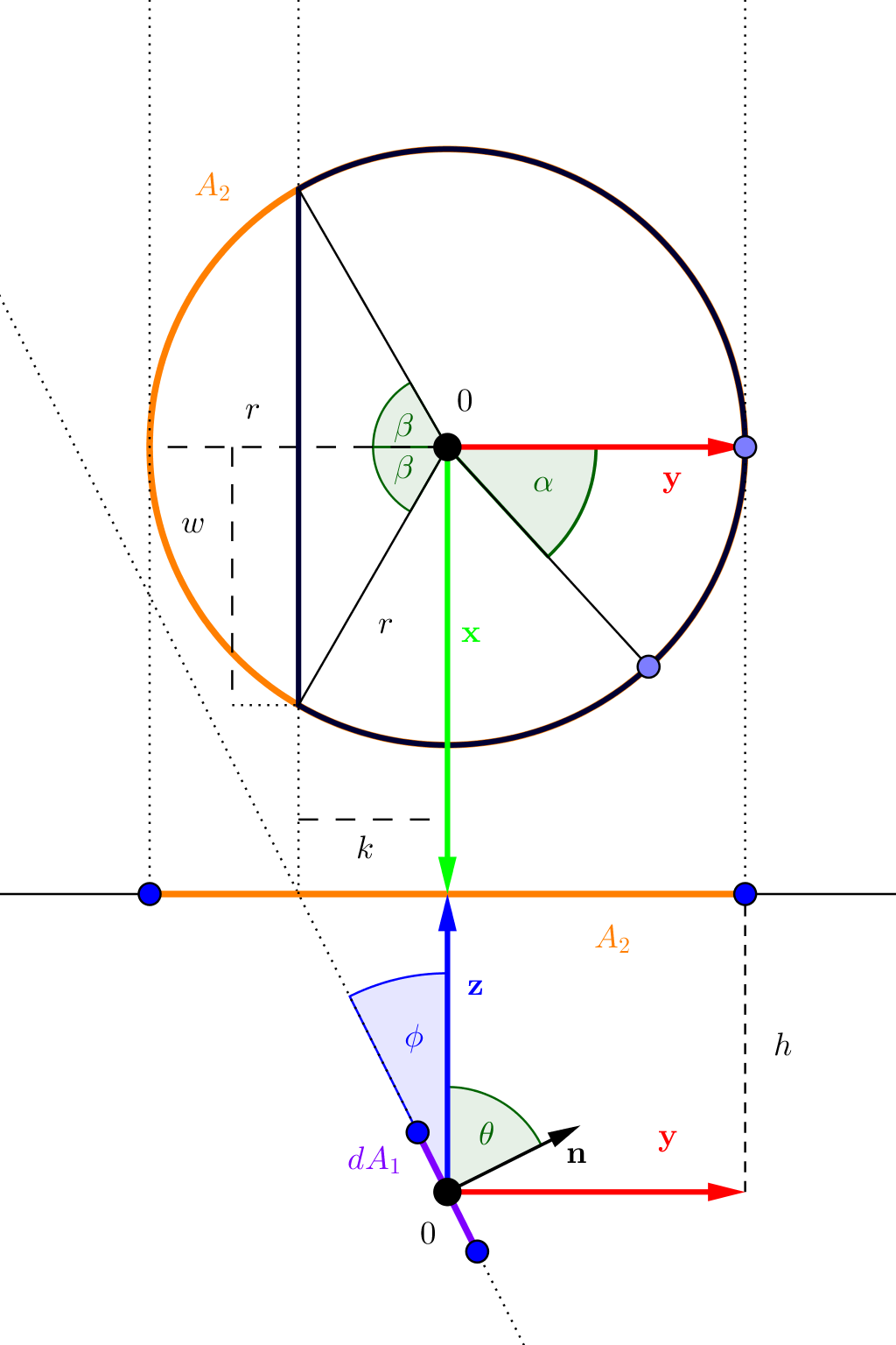
We want to compute the view factor of a disk and an oriented differential area located along the disk's normal. Before, we assumed all of the disk to be visible from our surface. But if our surface is rotated enough, the infinite plane it lies on intersects the disk. The cut off part is then behind the surface, so there is no radiation transfer. We will now handle that case. As before, we will derive the formula given in http://www.thermalradiation.net/sectionb/B-13.html. First a sketch of the updated setup:

The update from the last post is that we cut off the part of the disk behind the plane. The resulting shape is outlined in the very dark blue.

We will now find the condition for when the disk is fully visible. From the image, we can see that it is fully visible, if $k$ is larger than the disk's radius $r$. Since the normal is perpendicular to the plane, we have $\phi = \frac{\pi}{2} - \theta$. Computing the tangent yields:

$$\begin{aligned} \tan \phi &= \tan (\frac{\pi}{2} - \theta) \\ &= \cot \theta \\ &= \frac{k}{h} \end{aligned}$$

And following from that

$$k = h\cot \theta$$

For the visibility condition:

$$\begin{aligned} r \leq k \\r \leq h\cot \theta \\ \frac{r}{h} \leq \cot \theta \\ \cot^{-1}(\frac{r}{h}) \geq \theta \\ \cot^{-1}(\frac{1}{H}) \geq \theta \end{aligned}$$

The last line uses the definition $H = \frac{h}{r}$. The reversal of the inequality sign comes from the fact, that the inverse cotangent function is monotonically decreasing. This is the same condition as given in the reference. If it holds, we can apply the previous post's reasoning and are finished.

For the next steps we will compute $\beta$.

$$\begin{aligned} \cos \beta &= \frac{k}{r} \\ &= \frac{h\cot \theta}{r}\\ &= H\cot \theta \\ \beta &= \cos^{-1}(H\cot \theta) \end{aligned}$$

Since we will need it later, we can derive another useful expression with the identity $\sin(\cos^{-1}x) = \sqrt{1-x^2}$

$$\begin{aligned} \sin \beta &= \sin \cos^{-1}(H\cot \theta) \\ &= \sqrt{1-H^2\cot^2\theta} \\ &= X \end{aligned}$$

We will now proceed with the actual computation. It will be split into two parts, since the contour can be decomposed into two parts: A circle segment and a straight line.

Circle segment

Pretty much all the setup is the same as in the last part, so I will refer to that for more information. The only difference is the interval over which to integrate. Before we had the full circle in $[0,\pi]$. Now a part is missing. The new interval goes up to $\pi - \beta$ and starts at that value in negative $-(\pi - \beta) = -\pi + \beta$. One simplification can be done. Since the disk is symmetric, we could just integrate over half the disk and double the result. Doesn't matter in the end, just a bit less to write. We will now compute the values from before with the new bounds.

$$\begin{aligned} -\frac{hr\sin \theta}{2\pi(r^2+h^2)}*2 \int_0^{\pi - \beta} \cos \alpha d\alpha &= -\frac{hr\sin \theta}{\pi(r^2+h^2)}\int_0^{\pi - \beta} \cos \alpha d\alpha \\ &= -\frac{hr\sin \theta}{\pi(r^2+h^2)} (\sin(\pi - \beta) - \sin 0)\\ &= -\frac{hr\sin \theta}{\pi(r^2+h^2)}\sin(\beta) \\ &= -\frac{hr\sin \theta}{\pi(r^2+h^2)}X \\ &= -\frac{hrX\sin \theta}{\pi(r^2+h^2)} * \frac{r^2}{r^2}\\ &= -\frac{HX\sin \theta}{\pi(1+ H^2)} \end{aligned}$$

Then the second term:

$$\begin{aligned} \frac{r^2\cos \theta}{2\pi(r^2+h^2)}*2 \int_0^{\pi - \beta} 1 d\alpha &= \frac{r^2\cos \theta}{\pi(r^2+h^2)} \int_0^{\pi - \beta} 1 d\alpha \\ &= \frac{r^2\cos \theta}{\pi(r^2+h^2)} (\pi - \beta) \\ &= \frac{r^2\cos \theta}{\pi(r^2+h^2)}(\pi - \cos^{-1}(H\cot \theta))\\ &= \frac{\cos \theta}{\pi(1 + H^2)}(\pi - \cos^{-1}(H\cot \theta)) \end{aligned}$$

Line segment

The second contour segment is a line. We have computed a few values before:

$$\begin{aligned} l_1 &= 0\\ m_1 &= \sin \theta \\ n_1 &= \cos \theta \\ x_1 &= 0\\ y_1 &= 0 \\ z_1 &= 0 \end{aligned}$$

From our sketch we can see, that the line is constant in $z$ and $y$ direction and only varies in $x$. Instead of computing some line parametrization, we will just let $x_2$ vary from the line's start point to its endpoint. As before we will integrate over one half of the line and multiply the result by $2$. The half length of the line is given by $w$ in the sketch. We have to be careful not to change direction going around the contour. To comply with the winding direction of $\alpha$, we will vary the line from $w$ to $0$. Now on to compute $w$:

$$\begin{aligned} \sin \beta &= \frac{w}{r} \\ X &= \frac{w}{r} \\ w &= rX \end{aligned}$$

To compile all missing values:

$$\begin{aligned} x_2\\ y_2 &= -k = -h\cot \theta \\ z_2 &= h \end{aligned}$$

$$d^2 = x_2^2 + y_2^2 + z_2^2 = x_2^2 + h^2\cot^2\theta + h^2$$

$$\begin{aligned} dx_2\\ dy_2 &= 0 \\ dz_2 &= 0 \end{aligned}$$

In the following, we will use $1+\cot^2 \theta = \csc^2 \theta = \frac{1}{\sin^2 \theta}$ a few times. With that we also have $\sqrt{1+\cot^2\theta} = \frac{1}{\sin \theta}$. Also, just as a heads up, I will not go into the detail of the final explicit integration in each formula, as those can be acquired either from consulting something like WolframAlpha or integration tables. Just one reminder: $\tan^{-1}(0) = 0$. We have to compute the following expression:

$$\begin{aligned} &l_1\oint_C \frac{(z_2-z_1)dy_2 - (y_2-y_1)dz_2}{2\pi d^2} \\ &+ m_1\oint_C \frac{(x_2-x_1)dz_2 - (z_2-z_1)dx_2}{2\pi d^2} \\ &+ n_1\oint_C \frac{(y_2-y_1)dx_2 - (x_2-x_1)dy_2}{2\pi d^2} \end{aligned}$$

The first term is $0$, since $l_1=0$. Now on to solve the two remaining ones, keeping in mind the doubling of the result with half the line and the direction.

$$\begin{aligned}m_1\oint_C \frac{(x_2-x_1)dz_2 - (z_2-z_1)dx_2}{2\pi d^2} &= \frac{\sin \theta}{2\pi} * 2\int_{rX}^0 \frac{(x_2- 0)*0 - (h-0)dx_2}{x^2 + h^2\cot^2\theta +h^2} \\ &= \frac{\sin \theta}{\pi}\int_{rX}^0 \frac{- hdx_2}{x^2 + h^2\cot^2\theta +h^2} \\ &=\frac{h\sin \theta}{\pi}-\int_{0}^{rX} \frac{-dx_2}{x^2 + h^2\cot^2\theta +h^2} \\ &= \frac{h\sin \theta}{\pi}\int_{0}^{rX} \frac{dx_2}{x^2 + h^2\cot^2\theta +h^2} \\ &= \frac{h\sin \theta}{\pi}\frac{\tan^{-1}(\frac{x_2}{h\sqrt{1 + \cot^2\theta}})}{h\sqrt{1 + \cot^2\theta}}\rVert_0^{rX} \\ &= \frac{h\sin \theta}{\pi}\frac{\tan^{-1}(\frac{rX}{h\sqrt{1 + \cot^2\theta}})}{h\sqrt{1 + \cot^2\theta}} \\ &= \frac{\sin \theta}{\pi}\frac{\tan^{-1}(\frac{r}{h}\frac{X}{\frac{1}{\sin\theta}})}{\frac{1}{\sin \theta}} \\ &= \frac{\sin^2 \theta}{\pi}\tan^{-1}(\frac{1}{H}X\sin \theta) \\ &= \frac{\sin^2 \theta}{\pi}\tan^{-1}(\frac{X\sin \theta}{H}) \end{aligned}$$

Nearly done! Only one more to go! We will do some of the initial steps from the last one again in one go. Also, since there is a term $\cot\theta = \frac{\cos\theta}{\sin\theta}$ we do some rearranging.

$$\begin{aligned} n_1\oint_C \frac{(y_2-y_1)dx_2 - (x_2-x_1)dy_2}{2\pi d^2} &= \frac{\cos\theta}{2\pi}*2\int_{rX}^0 \frac{(-h\cot\theta -0)dx_2 - (x_2-0)*0}{x^2 + h^2\cot^2\theta +h^2}\\ &= \frac{h\cos\theta}{\pi}\int_{0}^{rX} \frac{\cot\theta dx_2}{x^2 + h^2\cot^2\theta +h^2}\\ &= \frac{h\cos\theta\cot\theta}{\pi}\int_{0}^{rX} \frac{dx_2}{x^2 + h^2(1+\cot^2\theta)}\\ &= \frac{h\cos\theta\cot\theta}{\pi}\int_{0}^{rX} \frac{dx_2}{x^2 + h^2(\frac{1}{\sin^2\theta})}\\ &= \frac{h\cos\theta\cot\theta}{\pi}\int_{0}^{rX} \frac{dx_2}{x^2 + h^2(\frac{1}{\sin^2\theta})}\frac{\sin^2\theta}{\sin^2\theta}\\ &= \frac{h\cos\theta\cos\theta\sin\theta}{\pi}\int_{0}^{rX} \frac{dx_2}{\sin^2\theta x^2 + h^2}\\ &= \frac{h\cos^2\theta \sin\theta}{\pi}\int_{0}^{rX} \frac{dx_2}{\sin^2\theta x^2 + h^2}\\ &= \frac{h\cos^2\theta \sin\theta}{\pi}\frac{\frac{1}{\sin \theta} \tan^{-1}(\frac{rX\sin \theta}{h})}{h}\\ &= \frac{\cos^2\theta }{\pi}\tan^{-1}(\frac{X\sin \theta}{H})\\ \end{aligned}$$

Wohoo! We can add the two results for the line:

$$\begin{aligned} \frac{\sin^2 \theta}{\pi}\tan^{-1}(\frac{X\sin \theta}{H}) + \frac{\cos^2\theta }{\pi}\tan^{-1}(\frac{X\sin \theta}{H}) &= \frac{1}{\pi}(cos^2\theta + \sin^2\theta) \tan^{-1}(\frac{X\sin \theta}{H}) \\ &=\frac{1}{\pi}\tan^{-1}(\frac{X\sin \theta}{H}) \end{aligned}$$

End result

The very last step now is to add the results for the circle segment and the line, which will result in the expression given in http://www.thermalradiation.net/sectionb/B-13.html:

$$\begin{aligned} F_{dA_1,A_2} &= -\frac{HX\sin \theta}{\pi(1+ H^2)} + \frac{\cos \theta}{\pi(1 + H^2)}(\pi - \cos^{-1}(H\cot \theta)) + \frac{1}{\pi}\tan^{-1}(\frac{X\sin \theta}{H}) \end{aligned}$$