Introduction

This document details the basic operations that arise when dealing with different coordinate systems. We will look at the special case of orthogonal, right-handed and unit-length basis vectors with a translation, as this is a very useful subset of coordinate transforms, that comes up in various fields and applications.

More general versions with scaling, or non-orthogonal basis vectors can be derived in a very similar way, though they lose a bit of the geometric intuition, so we don't cover them here.

Knowledge about vectors and matrix operations are needed.

Coordinate systems and transforms

A coordinate system $A$ can be described by its origin $\mathbf{o}_A$ and a set of $n$ basis vectors $\mathbf{x}_{A,i}, i=1,\dots, n$.

We require, that the basis vectors have a length of $1$ and are perpendicular to each other. This can be expressed with the dot product as:

$$\begin{aligned} \mathbf{x}_{A,i} \cdot \mathbf{x}_{A,j} &= \begin{cases} 1 & \text{, if }i = j\\ 0 & \text{, else}\end{cases} \\ &= \delta_i^j \end{aligned}$$

(The second line is the so called Kronecker delta and is just a shorthand for the brackets above)

Furthermore, they should form a right-handed coordinate system. This basically means, that the coordinate axes should "look like" the standard basis. In 2D, the $x$-axis points right and $y$ up. You can rotate these two around any angle, and they will still "look" the same. In 3D, the axes should conform to the right-hand-rule. In general n-D space, which includes the previous ones, we write the coordinate axes as rows or columns in a matrix and we call it right-handed, if that matrix has a determinant greater than zero (or exactly one in the case of our orthonormal system).

We imagine a point $\mathbf{p}$. This is a fixed point "in the world". In the coordinate system $A$ it can be described by its coordinates in that system $p^A_{i}$, where the index $\ _i^{A}$ corresponds to the associated basis vector $\mathbf{x}_{A,i}$. Geometrically, we move to the origin of $A$ ($\mathbf{o}_A$) and then continue to move $p^A_{i}$ units in the direction $\mathbf{x}_{A,i}$ for each $\mathbf{x}_{A,i}$. This can be written as:

$$\mathbf{p} = p^A_{1}\mathbf{x}_{A,1} + \dots + p^A_{n}\mathbf{x}_{A,n} + \mathbf{o}_A$$

A vector $\mathbf{v}$ does not have a fixed location in space, but just a direction and length. Therefore there is no addition of the origin.

$$\mathbf{v} = v^A_{1}\mathbf{x}_{A,1} + \dots + v^i_{n}\mathbf{x}_{A,n}$$

To see why that is, we can define a vector as the difference of two point $\mathbf{p} - \mathbf{q}$.

$$\begin{align*} \mathbf{v} &= \mathbf{p} - \mathbf{q} \\ &= p^A_{1}\mathbf{x}_{A,1} + \dots + p^A_{n}\mathbf{x}_{A,n} + \mathbf{o}_A - (q^A_{1}\mathbf{x}_{A,1} + \dots + q^A_{n}\mathbf{x}_{A,n} + \mathbf{o}_A)\\ &= p^A_{1}\mathbf{x}_{A,1} + \dots + p^A_{n}\mathbf{x}_{A,n} + \mathbf{o}_A - q^A_{1}\mathbf{x}_{A,1} - \dots + q^A_{n}\mathbf{x}_{A,n} - \mathbf{o}_A\\ &= (p^A_{1}- q^A_{1})\mathbf{x}_{A,1} + \dots + (p^A_{n}- q^A_n)\mathbf{x}_{A,n} \\ &= v^A_{1}\mathbf{x}_{A,1} + \dots + v^A_{n}\mathbf{x}_{A,n} \end{align*}$$

Taking the dot product of both sides with one of the axis vectors allows us to retrieve the individual coordinates, thanks to the property $\mathbf{x}_{A,i} \cdot \mathbf{x}_{A,j} = \delta_i^j$.

$$\begin{align*} \mathbf{p} &= p^A_{1}\mathbf{x}_{A,1} + \dots + p^A_{n}\mathbf{x}_{A,n} + \mathbf{o}_i\\ \mathbf{p} - \mathbf{o}_i &= p^A_{1}\mathbf{x}_{A,1} + \dots + p^A_{n}\mathbf{x}_{A,n} \\ \mathbf{x}_{A,i}\cdot (\mathbf{p} - \mathbf{o}_i) &= \mathbf{x}_{A,i}\cdot(p^A_{1}\mathbf{x}_{A,1} + \dots + p^A_{n}\mathbf{x}_{A,n})\\ &= p^A_{i} \\ \mathbf{v} &= v^A_{1}\mathbf{x}_{A,1} + \dots + v^A_{n}\mathbf{x}_{A,n}\\ \mathbf{x}_{A,i}\cdot \mathbf{v} &= \mathbf{x}_{A,i}\cdot(v^A_{1}\mathbf{x}_{A,1} + \dots + v^A_{n}\mathbf{x}_{A,n})\\ &= v^A_{i} \\ \end{align*}$$

This can be written in matrix notation with each $\mathbf{x}_{A,i}$ being a column and the coordinates $p^A_{i}$ forming a column vector $\mathbf{p}^A$. The upper index denotes the coordinates given in the system $A$.

$$\begin{align*} \mathbf{p} &= p^A_{1}\mathbf{x}_{A,1} + \dots + p^A_{n}\mathbf{x}_{A,n} + \mathbf{o}_A \\ &= \begin{pmatrix} \mathbf{x}_{A,1} & \dots & \mathbf{x}_{A,n} \end{pmatrix} \begin{pmatrix} p^A_{1} \\ \vdots \\ p^A_{n} \end{pmatrix} + \mathbf{o}_A \\ &= \mathbf{R}_A \mathbf{p}^A + \mathbf{o}_i\\ \mathbf{v} &= \mathbf{R}_A \mathbf{v}^A \end{align*}$$

We write which coordinate system the matrix $\mathbf{R}$ comes from as an index, here $\ _A$.

As the base vectors are normalized and orthogonal, the matrix $\mathbf{R}$ is a rotation matrix, which has the nice property, that $\mathbf{R}^{-1} = \mathbf{R}^T$. To actually calculate this, we will need to introduce some arbitrary coordinate system, in which we can express the $\mathbf{x}_{A,i}$ and $\mathbf{o}_A$. As there is no absolute coordinate frame, any choice is valid. You basically just need a way to measure your coordinates (or just being able to calculate the dot products between the axes and points or vectors! This means, you could geometrically construct your first coordinates!),

We can redo the extraction of the coordinates, but in matrix notation, this extracts the whole coordinate vector! To get the coordinate for one of the axes, we applied the axis with a dot product to the vector. If we just write all axes in the rows of a matrix and left multiply, that is exactly the same, but for all of them at once. But that is just $(\mathbf{R}_A)^T$. The resulting matrix of $(\mathbf{R}_A)^T\mathbf{R}_A$ contains all the pairwise dot products $\mathbf{x}_{A,i} \cdot \mathbf{x}_{A,j} = \delta_i^j$ and is thus the identity matrix. So we have:

$$\begin{align*} \mathbf{p} &= \mathbf{R}_A \mathbf{p}^A + \mathbf{o}_A\\ \mathbf{p} - \mathbf{o}_A &= \mathbf{R}_A \mathbf{p}^A \\ (\mathbf{R}_A)^T(\mathbf{p} - \mathbf{o}_A) &= (\mathbf{R}_A)^T \mathbf{R} \mathbf{p}^A \\ (\mathbf{R}_A)^T(\mathbf{p} - \mathbf{o}_A) &= \mathbf{p}^A \\ \mathbf{v} &= \mathbf{R}_A \mathbf{v}^A \\ (\mathbf{R}_A)^T\mathbf{v} &= (\mathbf{R}_A)^T\mathbf{R}_A \mathbf{v}^A \\ (\mathbf{R}_A)^T\mathbf{v} &= \mathbf{v}^A \\ \end{align*}$$

So applying $(\mathbf{R}_A)^T$ on the left hand side projects a vector onto the coordinate vectors of $A$!

We could also use non-normalized non-orthogonal axis vectors. In the calculations, we would just need to replace the transpose with the inverse when it comes up and everything still works the same. We can always find our special case axes though, for example with the Gram-Schmidt process. So in many practical cases, you might not want to deal with these more generic coordinate systems. So in the following, we will stick to the nicer version. Having dot products with orthogonal vectors also seems more geometrically easy to visualize. While you can construct stuff like the contravariant basis, this isn't really the focus here.

With that, we define a Transform. This isn't actually much different from the coordinate frame. From the last equations, we can see the base idea: A transform takes a coordinate vector defined in one coordinate system (start) $A$ and gives us the vector coordinates in the (target) system $B$ defined by the $\mathbf{x}_{B,i}$ with origin $\mathbf{o}_B$. We define a transform as the structure $\mathbf{T}_A^B = \{\mathbf{R}_A^B, \mathbf{t}_{A\rightarrow B}^B\}$ with the following semantics:

Given coordinates in the start system $A$, we can compute the coordinates in the target System $B$ with $\mathbf{T}_A^B$ according to:

$$\begin{align*} \mathbf{p}^B &= \mathbf{T}_A^B(\mathbf{p}^A) \\ &= \mathbf{R}_A^B \mathbf{p}^A + \mathbf{t}_{A\rightarrow B}^B \end{align*}$$

So a transform is a combination of a rotation and a translation of the coordinates. Writing the upper and lower indices in this way allows us to quickly check if we made a mistake, as multiplying a matrix will always have a matching lower index with the upper one of the coordinates. The translation $\mathbf{t}_{A\rightarrow B}^B$ represents the displacement that aligns the origin of $B$ with $A$ as expressed in the axes of $B$.

In fields like computer graphics, this is often combined into a single matrix (with higher dimension to allow for translation), as it allows for very easy concatenations of different operations by the usual matrix multiplication. We will not use that here, but the formulas can be easily converted. This can also include scaling and other linear transformations. You can also write it as multiple special matrices (rotation, scale, translation), which allows us to exploit the special structure of these matrices like this:

$$\begin{align*} \mathbf{T}_A^B &= \mathbf{T}_{\text{translation}}(\mathbf{t})\mathbf{R}\mathbf{S}_{\text{scale}}(\begin{pmatrix} s_1 \\ \vdots \\ s_n \end{pmatrix}) \\ (\mathbf{T}_A^B)^{-1} &= \mathbf{S}_{\text{scale}}(\begin{pmatrix} \frac{1}{s_1} \\ \vdots \\ \frac{1}{s_n} \end{pmatrix})\mathbf{R}^T\mathbf{T}_{\text{translation}}(\mathbf{-t}) \end{align*}$$

In this, you could also replace the rotation matrix by a unit quaternion, which has some nice properties.

One issue you will encounter with this, is that you have a hierarchy of coordinate systems with non-uniform scales and rotations, the full transform will not adhere to that definition, it will include some skewing! That is why you can't for example just retrieve a global scaling for an object in engines like Unity. So this setup only works locally (which is already very useful!)

In the next sections, we will look at the formulas to work with transforms. The sections include proofs, but you can skip them if you are not interested and just want to use or check the formulas.

Defining a transform based on two coordinate systems

We are given a start coordinate system $A$ and a target $B$. The transform that transforms point coordinates from $A$ to $B$ according to $\mathbf{p}^B = \mathbf{R}_A^B \mathbf{p}^A + \mathbf{t}_{A\rightarrow B}^B$ is given by:

$$\begin{align*} \mathbf{R}_A^B &= \begin{pmatrix}(\mathbf{x}_{B,1})^T \\ \vdots \\ (\mathbf{x}_{B,n})^T\end{pmatrix} \begin{pmatrix}\mathbf{x}_{A,1} & \dots & \mathbf{x}_{A,n}\end{pmatrix} \\ &= (\mathbf{R}_B)^T\mathbf{R}_A\\ \mathbf{t}_{A\rightarrow B}^B &= \begin{pmatrix}(\mathbf{x}_{B,1})^T \\ \vdots \\ (\mathbf{x}_{B,n})^T\end{pmatrix} (\mathbf{o}_A - \mathbf{o}_B)\\ &= (\mathbf{R}_B)^T(\mathbf{o}_A - \mathbf{o}_B) \end{align*}$$

The upper index $\ ^B$ comes from the fact that $(\mathbf{R}_B)^T$ by definition transforms a vector into the coordinates of $B$.

Important: The basis vector and origin coordinates of the two coordinate systems must be expressed in the same system. As stated before, this is arbitrary and could be any system we like. One could for example express both systems as seen from $A$. This would lead to the simplification: $\begin{pmatrix}\mathbf{x}_{A,1}^A & \dots & \mathbf{x}_{A,n}^A\end{pmatrix} = \mathbf{I}_n$ ($\mathbf{I}_n$ is the identity matrix) and $\mathbf{o}_A= \mathbf{0}$.

This special case leads to:

$$\begin{align*} \mathbf{R}_A^B &= \begin{pmatrix}(\mathbf{x}_{B,1}^A)^T \\ \vdots \\ (\mathbf{x}_{B,n}^A)^T\end{pmatrix} \\ &= (\mathbf{R}_B)^T\\ \mathbf{t}_{A\rightarrow B}^B &= \begin{pmatrix}(\mathbf{x}_{B,1}^A)^T \\ \vdots \\ (\mathbf{x}_{B,n}^A)^T\end{pmatrix} (-\mathbf{o}_B^A)\\ &= -\mathbf{R}_A^B\mathbf{o}_B^A \end{align*}$$

This is a common formula found for example in the camera coordinate system transform in computer graphics. First you move to the center ($-\mathbf{o}_B^A$) and then you project onto the camera axes. This projection comes from $\mathbf{R}_A^B$ which contains the axis vectors in its rows. Multiplying a vector to the right is equivalent to computing the dot product with each axis vector. Since the vectors are normalized and perpendicular, this lets us know "how much" our vector points in the direction of one of the axes. This amount is just a coordinate. As a $n+1$ dimensional (we need one extra dimension to fit in the translation) matrix product this is:

$$\begin{align*} \underbrace{\mathbf{R}_{B}}_{\text{Rotation}}\underbrace{\mathbf{T}(-\mathbf{o}_B^A)}_{\text{Translation}} &= \left(\begin{array}{c|c} (\mathbf{x}_{B,1})^T & 0 \\ \vdots & \vdots \\ (\mathbf{x}_{B,n})^T & 0 \\\hline \mathbf{0}^T & 1 \end{array}\right) \left(\begin{array}{c|c} \mathbf{I}_n & -\mathbf{o}_B^A \\\hline \mathbf{0}^T & 1 \end{array}\right) \\ &= \left(\begin{array}{c|c} \mathbf{R}_{A}^B & 0 \\\hline \mathbf{0}^T & 1 \end{array}\right) \left(\begin{array}{c|c} \mathbf{I}_n & -\mathbf{o}_B^A \\\hline \mathbf{0}^T & 1 \end{array}\right)\\ &= \left(\begin{array}{c|c} \mathbf{R}_{A}^B & -\mathbf{R}_{A}^B\mathbf{o}_B^A \\\hline \mathbf{0}^T & 1 \end{array}\right) \end{align*}$$

Proof

We can describe the point $\mathbf{p}$ using our two coordinate systems $A$ and $B$. From before we know how to express a point with local coordinates:

$$\begin{align*} \mathbf{p} &= \begin{pmatrix} \mathbf{x}_{A,1} & \dots & \mathbf{x}_{A,n} \end{pmatrix} \mathbf{p}^A + \mathbf{o}_A \\ &= \mathbf{R}_A \mathbf{p}^A + \mathbf{o}_A\\ \mathbf{p} &= \begin{pmatrix} \mathbf{x}_{B,1} & \dots & \mathbf{x}_{B,n} \end{pmatrix} \mathbf{p}^B + \mathbf{o}_B \\ &= \mathbf{R}_B \mathbf{p}^B + \mathbf{o}_B\\ \end{align*}$$

Just to restate: The point itself does not change, we just use different coordinates appropriate for each system. We can equate both equations and then solve for $\mathbf{p}^B$, which will leave us with a transform expression.

$$\begin{align*} \mathbf{R}_A\mathbf{p}^A + \mathbf{o}_A &= \mathbf{R}_B \mathbf{p}^B + \mathbf{o}_B \\ \mathbf{R}_A\mathbf{p}^A + \mathbf{o}_A - \mathbf{o}_B&= \mathbf{R}_B \mathbf{p}^B \\ (\mathbf{R}_B)^T\mathbf{R}_A \mathbf{p}^A + (\mathbf{R}_B)^T(\mathbf{o}_A - \mathbf{o}_B)&= (\mathbf{R}_B)^T \mathbf{R}_B \mathbf{p}^B \\ (\mathbf{R}_B)^T\mathbf{R}_A \mathbf{p}^A + (\mathbf{R}_B)^T(\mathbf{o}_A - \mathbf{o}_B)&= \mathbf{I}_n \mathbf{p}^B \\ \underbrace{ (\mathbf{R}_B)^T\mathbf{R}_A}_{\mathbf{R}_A^B} \mathbf{p}^A + \underbrace{(\mathbf{R}_B)^T(\mathbf{o}_A - \mathbf{o}_B)}_{\mathbf{t}_{A\rightarrow B}^B} &= \mathbf{p}^B \\ \mathbf{R}_A^B \mathbf{p}^A + \mathbf{t}_{A\rightarrow B}^B &= \mathbf{p}^B \end{align*}$$

The identity matrix comes again from the fact, that $\mathbf{x}_{B,i} \cdot \mathbf{x}_{B,j} = \delta_i^j$ or alternatively, that the matrix formed by the basis vectors is a rotation matrix, with the transpose being its inverse, as stated previously.

$\mathbf{R}_A^B$ is the product of two rotation matrices and thus is a rotation matrix itself. This property is easy to check.

$$\begin{align*} (\mathbf{R}_A^B)^T\mathbf{R}_A^B &= ((\mathbf{R}_B)^T\mathbf{R}_A)^T (\mathbf{R}_B)^T\mathbf{R}_A \\ &= (\mathbf{R}_A)^T\mathbf{R}_B (\mathbf{R}_B)^T\mathbf{R}_A \\ &= (\mathbf{R}_A)^T(\mathbf{R}_B (\mathbf{R}_B)^T)\mathbf{R}_A \\ &= (\mathbf{R}_A)^T\mathbf{I}\mathbf{R}_A \\ &= (\mathbf{R}_A)^T\mathbf{R}_A \\ &= \mathbf{I} \end{align*}$$

Furthermore, the determinant is one, since $\mathrm{det}{\mathbf{R}_A^B} =\mathrm{det}{((\mathbf{R}_B)^T\mathbf{R}_A)} =\mathrm{det}{(\mathbf{R}_B)^T}\mathrm{det}{\mathbf{R}_A}= 1 * 1 = 1$.

Next, we will check, that the computed transform is independent of the coordinate axes that we express our axes in (if at all in one).

We can compute, as seen before, the coordinates of the axis vector $\mathbf{x}_{A,i}$ for the coordinate system $W$ as $\mathbf{x}_{A,i}^W = (\mathbf{R}_W)^T\mathbf{x}_{A,i}$. The same is true for $\mathbf{x}_{B,i}$. The coordinate origin coordinates are found by $\mathbf{o}_{A}^W = (\mathbf{R}_W)^T(\mathbf{o}_{A} - \mathbf{o}_W)$ with $\mathbf{o}_B^W$ being handled the same again. Doing that for all the axes gathered in the columns of $\mathbf{R}_A$ (and similarly $\mathbf{R}_B$):

$$\begin{align*} \mathbf{R}_A^W &= (\mathbf{R}_W)^T \mathbf{R}_A\\ \mathbf{R}_W\mathbf{R}_A^W &= \underbrace{\mathbf{R}_W(\mathbf{R}_W)^T}_{\mathbf{I}}\mathbf{R}_A \\ \mathbf{R}_W\mathbf{R}_A^W &= \mathbf{R}_A \\ \mathbf{o}_A^W &= (\mathbf{R}_W)^T\mathbf{o}_A + \mathbf{o}_W \\ \mathbf{R}_W\mathbf{o}_A^W &= \underbrace{\mathbf{R}_W(\mathbf{R}_W)^T}_{\mathbf{I}}\mathbf{o}_A + \mathbf{o}_W \\ \mathbf{R}_W\mathbf{o}_A^W &= \mathbf{o}_A + \mathbf{o}_W\\ \mathbf{R}_W\mathbf{o}_A^W -\mathbf{o}_W &= \mathbf{o}_A \end{align*}$$

Note that the notation $\mathbf{R}_A^W$ is used, since $(\mathbf{R}_W)^T \mathbf{R}_A$ follows the exact same definition that we used for $\mathbf{R}_A^B$. This means, that this product just represents the projection of $A$'s axes onto the axes of $W$ (and similarly for any system in the lower index that is projected onto the upper one). So $\mathbf{R}_A^W$ are the coordinates of $A$'s axes in the the system $W$.

Furthermore, the notation also works, if the axes are just given as abstract vectors, in that case we just leave the index blank! For example, $\mathbf{R}_A$ transforms point coordinates from $A$ into the "geometric space".

We can use this in our found formula for the transform elements.

$$\begin{align*} \mathbf{R}_A^B &= (\mathbf{R}_B)^T\mathbf{R}_A \\ &= (\mathbf{R}_W\mathbf{R}_B^W)^T\mathbf{R}_W\mathbf{R}_A^W \\ &= (\mathbf{R}_B^W)^T\underbrace{(\mathbf{R}_W)^T\mathbf{R}_W}_{\mathbf{I}}\mathbf{R}_A^W \\ &= (\mathbf{R}_B^W)^T\mathbf{R}_A^W\\ \mathbf{t}_{A\rightarrow B}^B &= (\mathbf{R}_B)^T (\mathbf{o}_A - \mathbf{o}_B) \\ &= (\mathbf{R}_W\mathbf{R}_B^W)^T(\mathbf{R}_W\mathbf{o}_A^W -\mathbf{o}_W - (\mathbf{R}_W\mathbf{o}_B^W -\mathbf{o}_W)) \\ &= (\mathbf{R}_W\mathbf{R}_B^W)^T(\mathbf{R}_W\mathbf{o}_A^W -\mathbf{o}_W - \mathbf{R}_W\mathbf{o}_B^W +\mathbf{o}_W) \\ &= (\mathbf{R}_W\mathbf{R}_B^W)^T(\mathbf{R}_W\mathbf{o}_A^W - \mathbf{R}_W\mathbf{o}_B^W ) \\ &= (\mathbf{R}_W\mathbf{R}_B^W)^T\mathbf{R}_W(\mathbf{o}_A^W - \mathbf{o}_B^W ) \\ &= (\mathbf{R}_B^W)^T\underbrace{(\mathbf{R}_W)^T\mathbf{R}_W}_{\mathbf{I}}(\mathbf{o}_A^W - \mathbf{o}_B^W ) \\ &= (\mathbf{R}_B^W)^T(\mathbf{o}_A^W - \mathbf{o}_B^W ) \\ \end{align*}$$

So the formulas stay exactly the same, regardless in which coordinate system we express the points and vectors in, as long as that system is the same for all of them.

For the special case, we just want to check, that the local coordinates of the axes are the standard basis vectors (zeros everywhere, aside from the index of the axis, where there is a 1). We call this standard vector $\mathbf{e}_i = \begin{pmatrix} 0_0 \\ \vdots \\ 1_i \\ \vdots \\0_n \end{pmatrix}$

The $i$-th basis vector of the coordinate system $A$ is given as $\mathbf{x}_{A,i}$. Writing this as a matrix product:

$$\begin{align*} \mathbf{x}_{A,i} &= \begin{pmatrix} \mathbf{x}_{A,1} & \dots & \mathbf{x}_{A,n} \end{pmatrix} \begin{pmatrix} 0_0 \\ \vdots \\ 1_i \\ \vdots \\0_n \end{pmatrix} \\ &= \mathbf{R}_A\mathbf{e}_i \end{align*}$$

Computing the local coordinates in $A$ by applying $(\mathbf{R}_A)^T$:

$$\begin{align*} \mathbf{x}_{A,i}^A &= (\mathbf{R}_A)^T\mathbf{x}_{A,i} \\ &= (\mathbf{R}_A)^T\mathbf{R}_A\mathbf{e}_i \\ &= \mathbf{I}\mathbf{e}_i\\ &= \mathbf{e}_i \end{align*}$$

So, if we write all of these in the columns of a matrix as before, we get the rotation matrix expressed in the coordinate system $A$: $\mathbf{R}_A^A = \mathbf{I}$

The notation stays consistent here: This matrix transforms coordinates from $A$ to $A$, so they are unchanged!

Next up, let's calculate the origin $\mathbf{o}_A$ in the coordinates of $A$, namely $\mathbf{o}_A^A$. From the formula to get coordinates of a point we have:

$$\begin{align*} \mathbf{o}_A^A &= (\mathbf{R}_A)^T(\mathbf{o}_a - \mathbf{o}_a) \\ &= \mathbf{0} \end{align*}$$

Thus the origin of $A$ in the coordinates of $A$ is, as probably expected, the zero vector $\mathbf{0}$.

We can now return to the special case. Expressing all points and vectors in the transform $\mathbf{T}_A^B$ in the coordinates of $A$ gives us:

$$\begin{align*} \mathbf{R}_A^B &= (\mathbf{R}_B^A)^T\mathbf{R}_A^A\\ &= (\mathbf{R}_B^A)^T\mathbf{I} \\ &= (\mathbf{R}_B^A)^T\\ \mathbf{t}_{A\rightarrow B}^B &= (\mathbf{R}_B^A)^T(\mathbf{o}_A^A - \mathbf{o}_B^A ) \\ &= (\mathbf{R}_B^A)^T(\mathbf{0} - \mathbf{o}_B^A ) \\ &= -(\mathbf{R}_B^A)^T \mathbf{o}_B^A \\ &= -\mathbf{R}_A^B \mathbf{o}_B^A \\ \end{align*}$$

Inverse of a transform

The inverse $\mathbf{T}_B^A = (\mathbf{T}_A^B)^{-1}$ of a given transform $\mathbf{T}_A^B$ is given by:

$$\begin{align*} \mathbf{R}_B^A &= (\mathbf{R}_A^B)^T \\ \mathbf{t}_{B\rightarrow A}^A &= -(\mathbf{R}_A^B)^T\mathbf{t}_{A\rightarrow B}^B \\ &= -\mathbf{R}_B^A\mathbf{t}_{A\rightarrow B}^B \end{align*}$$

The transform transforms a point from $B$ to $A$.

Proof

We start from the transformation equation: $\mathbf{p}^B = \mathbf{R}_A^B \mathbf{p}^A + \mathbf{t}_{A\rightarrow B}^B$. We just have to solve for $\mathbf{p}^A$.

$$\begin{align*} \mathbf{p}^B &= \mathbf{R}_A^B \mathbf{p}^A + \mathbf{t}_{A\rightarrow B}^B \\ \mathbf{p}^B - \mathbf{t}_{A\rightarrow B}^B &= \mathbf{R}_A^B \mathbf{p}^A \\ (\mathbf{R}_A^B)^T(\mathbf{p}^B - \mathbf{t}_{A\rightarrow B}^B) &= (\mathbf{R}_A^B)^T\mathbf{R}_A^B \mathbf{p}^A \\ \underbrace{(\mathbf{R}_A^B)^T}_{\mathbf{R}_B^A}\mathbf{p}^B \underbrace{- (\mathbf{R}_A^B)^T\mathbf{t}_{A\rightarrow B}^B}_{\mathbf{t}_{B\rightarrow A}^A} &= \mathbf{p}^A \\ \mathbf{R}_B^A \mathbf{p}^B + \mathbf{t}_{B\rightarrow A}^A &= \mathbf{p}^A \end{align*}$$

Composing two transforms

We can compose a transform $\mathbf{T}_A^M$ (from $A$ to $M$) and another transform $\mathbf{T}_M^B$ (from $M$ to $B$) to get $\mathbf{T}_A^B$ (from $A$ to $B$) as follows:

$$\begin{align*} \mathbf{R}_A^B &= \mathbf{R}_M^B\mathbf{R}_A^M \\ \mathbf{t}_{A\rightarrow B}^B &= \mathbf{R}_M^B\mathbf{t}_{A\rightarrow M}^M + \mathbf{t}_{M\rightarrow B}^B \\ &=\mathbf{T}_M^B (\mathbf{t}_{A\rightarrow M}^M ) \end{align*}$$

We write this composition simply as:

$$\mathbf{T}_A^B = \mathbf{T}_M^B\mathbf{T}_A^M$$

Note, that the order is from right to left.

Taking a look at the inverse composed transform, we can see, that it follows the same rules as matrix multiplications. The inverse of a composed ("multiplied") transform is the composition ("product") of the inverses of its parts in reverse order.

$$\begin{align*} (\mathbf{T}_A^B)^{-1} &= \mathbf{T}_B^A\\ &= \mathbf{T}_M^A\mathbf{T}_B^M \\ &= (\mathbf{T}_A^M)^{-1}(\mathbf{T}_M^B)^{-1} \end{align*}$$

As this section is the core of this document, there is also a quick example coming up on how to apply it.

Example

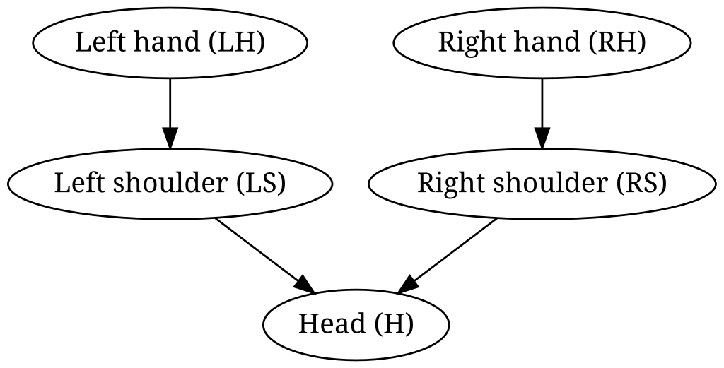
To give you an example how this is applicable, let's look at a simplified hierarchy of coordinate systems, that you could find in a part a humanoid animation rig or robot.

The direction of the arrows indicate how our local transformations are defined. Basically, we define a transformation, that takes us from a child to the parent. That way a child only needs to know how it is rotated and translated with respect to its parent. Therefore, we have four transforms:

• $\mathbf{T}_{\text{LH}}^{\text{LS}}$
• $\mathbf{T}_{\text{LS}}^{\text{H}}$
• $\mathbf{T}_{\text{RH}}^{\text{RS}}$
• $\mathbf{T}_{\text{RS}}^{\text{H}}$

We can now use our rules to construct the transformation that transforms points from the left hand to the right hand!

When we look at the tree above, we can try to find a path from left to right hand. In this case it is pretty easy, since the hierarchy is easy.

Left hand -> Left shoulder -> Head -> Right Shoulder -> Right hand.

Now we try to express that in transformations. With our index notation, this isn't too hard. We are looking for $\mathbf{T}_{\text{LH}}^{\text{RH}}$. Since the order is from right to left, we know that the upper index on the left will be $\text{RH}$ and the lower one on the right $\text{LH}$. From the sequence above, we can then just fill in the intermediate ones.

To make writing a bit easier, we can also split this into two parts: Left hand -> Head and Head -> Right hand.

$$\begin{align*} \mathbf{T}_{\text{LH}}^{\text{H}} &= \mathbf{T}_{\text{LS}}^{\text{H}}\mathbf{T}_{\text{LH}}^{\text{LS}} \\ \mathbf{T}_{\text{H}}^{\text{RH}} &= \mathbf{T}_{\text{RS}}^{\text{RH}}\mathbf{T}_{\text{H}}^{\text{RS}} \\ &= (\mathbf{T}_{\text{RH}}^{\text{RS}})^{-1}(\mathbf{T}_{\text{RS}}^{\text{H}})^{-1} \\ \end{align*}$$

Then the final transform is just:

$$\begin{align*} \mathbf{T}_{\text{LH}}^{\text{RH}} &= \mathbf{T}_{\text{H}}^{\text{RH}}\mathbf{T}_{\text{LH}}^{\text{H}} \\ &= \mathbf{T}_{\text{RS}}^{\text{RH}}\mathbf{T}_{\text{H}}^{\text{RS}}\mathbf{T}_{\text{LS}}^{\text{H}}\mathbf{T}_{\text{LH}}^{\text{LS}}\\ &= (\mathbf{T}_{\text{RH}}^{\text{RS}})^{-1}(\mathbf{T}_{\text{RS}}^{\text{H}})^{-1}\mathbf{T}_{\text{LS}}^{\text{H}}\mathbf{T}_{\text{LH}}^{\text{LS}} \end{align*}$$

We have expressed the full transform with only our initially known transforms. Now we need to apply the inverse and compose rules to each part and we get the final values.

This is something you see in most game engines, where you can define an object hierarchy, in 3D rigging, in robots and many more applications.

You just need to find the shortest (or actually any) path in the hierarchy between your desired start and target systems. In the easiest way, you start with your start transform and traverse the path, at each step applying the composition with the next node. Depending on whether you traveled along or against the direction of the graph array, the composition will take the transform itself (for example from left hand to left shoulder) or the inverse (for example from the head to the right shoulder).

With that, you will have implemented a generic coordinate transformation system!

Proof

For the proof, we just successively apply both transforms.

$$\begin{align*} \mathbf{p}^M &= \mathbf{T}_A^M (\mathbf{p}^A)\\ \mathbf{p}^B &= \mathbf{T}_M^B(\mathbf{p}^M) \\ &= \mathbf{T}_M^B(\mathbf{T}_A^M (\mathbf{p}^A)) \\ &= \mathbf{T}_M^B(\mathbf{R}_A^M \mathbf{p}^A + \mathbf{t}_{A\rightarrow M}^M ) \\ &= \mathbf{R}_M^B(\mathbf{R}_A^M \mathbf{p}^A + \mathbf{t}_{A\rightarrow M}^M ) + \mathbf{t}_{M\rightarrow B}^B \\ &= \underbrace{\mathbf{R}_M^B\mathbf{R}_A^M}_{\mathbf{R}_A^B} \mathbf{p}^A + \underbrace{\mathbf{R}_M^B\mathbf{t}_{A\rightarrow M}^M + \mathbf{t}_{M\rightarrow B}^B}_{\mathbf{t}_{A\rightarrow B}^B} \\ &= \mathbf{R}_A^B\mathbf{p}^A + \mathbf{t}_{A\rightarrow B}^B \end{align*}$$

Transforming points and vectors

The transform $\mathbf{T}_A^B$ transforms point coordinates from $A$ to $B$.

By definition, point coordinates are transformed as:

$$\mathbf{p}^B = \mathbf{R}_A^B \mathbf{p}^A + \mathbf{t}_{A\rightarrow B}^B$$

Vectors $\mathbf{v}^A$ have no position in space and thus do not use the translation part.

$$\mathbf{v}^B = \mathbf{R}_A^B \mathbf{v}^A$$

Proof

The point formula is just the definition of the transform.

We already showed that the projection for vectors does not include the translational part, but we will write it again with the transform formula.

For the vector $\mathbf{v}^A$, we consider that it can be defined by two points $\mathbf{p}^A$ and $\mathbf{q}^A$ as $\mathbf{v}^A =\mathbf{p}^A - \mathbf{q}^A$. In the $B$ coordinate system, the vector is of course still defined by the same points, but in $B$ coordinates ($\mathbf{p}^B, \mathbf{q}^B$). Since we know how points transform, we just plug it in.

$$\begin{align*} \mathbf{v}^B &= \mathbf{p}^B - \mathbf{q}^B \\ &= \mathbf{R}_A^B\mathbf{p}^A + \mathbf{t}_{A\rightarrow B}^B - (\mathbf{R}_A^B\mathbf{q}^A + \mathbf{t}_{A\rightarrow B}^B) \\ &= \mathbf{R}_A^B\mathbf{p}^A + \mathbf{t}_{A\rightarrow B}^B - \mathbf{R}_A^B\mathbf{q}^A - \mathbf{t}_{A\rightarrow B}^B \\ &= \mathbf{R}_A^B\mathbf{p}^A - \mathbf{R}_A^B\mathbf{q}^A \\ &= \mathbf{R}_A^B (\mathbf{p}^A - \mathbf{q}^A) \\ &= \mathbf{R}_A^B \mathbf{v}^A \\ \end{align*}$$

Retrieving coordinate axes

We can get information about the start and target coordinate axes from the rotation matrix $\mathbf{R}_A^B$ of a transform.

The $i$-th column is the $i$-th basis vector of $A$ in coordinates of $B$.

The $i$-th row is the $i$-th basis vector of $B$ in coordinates of $A$.

Proof

This is basically what we have already shown. The $j$-th coordinate of the $i$-th axis $\mathbf{x}_{A,i}$ of $A$ in $B$ is found by projecting the vector onto $\mathbf{x}_{B,j}$: $\mathbf{x}_{A,i} \cdot \mathbf{x}_{B,j}$.

Writing all of $B$'s axis vectors into the rows of a matrix and multiplying with $\mathbf{x}_{A,i}$ then gives us the full coordinate vector $\mathbf{x}_{A,i}^B$.

$$\begin{align*} \mathbf{x}_{A,i}^B &= \begin{pmatrix} (\mathbf{x}_{B,0})^T \\ \vdots \\ (\mathbf{x}_{B,n})^T \end{pmatrix} \mathbf{x}_{A,i} \\ &= (\mathbf{R}_B)^T \mathbf{x}_{A,i} \end{align*}$$

Writing all $\mathbf{x}_{A,i}$ in the columns of a matrix and multiplying by $(\mathbf{R}_{B})^T$ on the left is then equal to multiplying $(\mathbf{R}_{B})^T$ by each $\mathbf{x}_{A,i}$ and writing the resulting vectors into a new matrix.

$$\begin{align*} \begin{pmatrix} \mathbf{x}_{A,0}^B && \dots && \mathbf{x}_{A,n}^B \end{pmatrix} &= \begin{pmatrix} (\mathbf{R}_{B})^T \mathbf{x}_{A,0} && \dots && (\mathbf{R}_{B})^T \mathbf{x}_{A,n} \end{pmatrix} \\ &= (\mathbf{R}_{B})^T\begin{pmatrix} \mathbf{x}_{A,0} && \dots && \mathbf{x}_{A,n} \end{pmatrix} \\ &= (\mathbf{R}_{B})^T \mathbf{R}_A \\ &= \mathbf{R}_A^B \end{align*}$$

Thus we have shown, that the columns of $\mathbf{R}_A^B$ contain the axes of $A$ as expressed in $B$.

By the same logic, we know that $\mathbf{R}_B^A$ contains the axes of $A$ as expressed in $B$. But we have already shown, that $\mathbf{R}_B^A = (\mathbf{R}_A^B)^T$. Thus, the columns of $\mathbf{R}_B^A$ are just the rows of $\mathbf{R}_A^B$, which was the second statement.

Interactive demo

The following demo allows you to visually inspect the coordinate transform between two coordinate systems $A$ and $B$. You can move around the systems by dragging the gray dots. You can also move the black point $\mathbf{p}$.

The coordinates of $\mathbf{p}$ in the coordinate systems are displayed (can be disabled), so you can check the values.

Technically, we start by defining all the axes and points in the shared "world" coordinate system. We regard this as the default here and won't specifically annotate every vector with a $W$.

Below, the full transformation with all formulas is computed, if you want to check those as well. When cross-checking with the image, just keep in mind that there might sometimes be a slight discrepancy in the decimals due to rounding.