Sampling directions and normals for path tracing
Introduction
This document is meant as both a quick reference as well as documentation of a few sampling techniques that can be used in path tracing. It mostly came about because I found it hard to find such a reference or the derivations themselves.
This is of course not every kind of sampling technique (for example, no stratified sampling) or distribution, just a few, but maybe someone else can use it as well.
Each Sampling method will have the algorithm and probability density functions listed first and afterwards a derivation. So if you are just looking up how to implement it, you can find it below the images. The images (for the 3D directions) show a heatmap hemisphere corresponding to a number of samples chosen with the showcased method. The heatmap values correspond to number of points per area. Regions with high values will receive more samples than regions with low values.
In general I tried to include every step in the derivation so hopefully it is easy enough to follow.
This document is created as a python notebook to create the graphics and have the generating code together with the written out formulas. Please don’t be too hard on my python code, I am not the biggest python fan and just wanted it to work :’)
- Introduction
- Inverse Transform Sampling
- Sampling 2D
- Sampling Hemisphere Directions
- Sampling Distribution Of Normals
import matplotlib.pyplot as plt
import numpy as np
import math
from matplotlib import cm, colors
# general size parameters
plt.rcParams["figure.figsize"]=20,20
plt.rcParams.update({'font.size': 22})
# heatmap visualization parameters

# number of sample points per hemisphere
N = 10000000

# hemisphere resolution
hemi_res = 40
def hemisphereheatmap(theta, phi, res):
    # used for geometry
    phis = np.linspace(0, 2*np.pi, res)
    thetas = np.linspace(0, np.pi/2, res)
    T, P = np.meshgrid(thetas, phis)
    rs = np.zeros(np.shape(P))

    dt = thetas[1] - thetas[0]
    dp = phis[1] - phis[0]


    # sort calculated values into the hemisphere bins
    t = np.clip(np.floor(theta / (np.pi/2)*res),0,res-1).astype(int)
    p = np.clip(np.floor(phi / (np.pi*2)*res),0,res-1).astype(int)

    # count bins
    for i in range(len(theta)):
        ti = t[i]
        pi = p[i]

        rs[pi,ti] += 1

    for ti in range(res):
        for pi in range(res):
            # calculate the area of a patch to normalize points per area
            a = dp * (math.cos(thetas[ti]) - math.cos(thetas[ti] + dt))
            if a != 0:
                rs[pi,ti] /= math.fabs(a)
    rs /= np.max(rs)

    x = np.sin(T) * np.cos(P)
    y = np.sin(T) * np.sin(P)
    z = np.cos(T)
    ax = plt.figure().add_subplot(111, projection='3d')
    ax.plot_surface(x, y, z,  vmin=0,rstride=1, cstride=1,facecolors=cm.viridis(rs))
    ax.set_xlim(-1,1)
    ax.set_ylim(-1,1)
    ax.set_zlim(-1,1)
    ax.set_box_aspect([1,1,1])
    # add colorbar
    m = cm.ScalarMappable(cmap=cm.viridis)
    m.set_array([])
    plt.colorbar(m)

    return ax
Inverse Transform Sampling
The following sections will explore some ways to sample points/directions used for the Monte Carlo integration. The recipe for calculating the sampling formulas is called inverse transform sampling (there are, of course, other methods)
- Generate a uniform random number in the interval \([0,1]\)
- Find the cumulative distribution function (CDF) \(P\) of the desired distribution \(p\)
- Calculate \(v=P^{-1}(u)\). \(v\) will be distributed with \(p\)
Since we usually need two-dimensional values, we have to modify it a bit
- Generate two uniform random numbers \(u_1, u_2\) in the interval \([0,1]\)
- The probability density function \(p\) is dependent on \(x_1, x2\), so \(p(x_1,x_2)\)
- Calculate the marginal distribution \(p_{x_1}(x1)= \int_{\Omega_2}p(x1,x2)dx_2\)
- Calculate the conditional probability distribution of \(x_2\) with respect to \(x_1\) with the Bayes theorem: \(p(x2\vert x1)=p(x_1,x_2)p_{x_1}(x_1)\)
- Calculate the CDFs \(P_{x_1}(x_1)\) and \(P{x_2}(x_2)\).
- Calculate \(v_1=P_{x_1}^{-1}(u_1)\) and \(v_2=P_{x_2}^{-1}(u_2)\) . \(v_1\) and \(v_2\) will have the desired distribution
(see for example: https://www.slac.stanford.edu/slac/sass/talks/MonteCarloSASS.pdf)
Sampling 2D
To start of, we sample a 2D circle/disc.
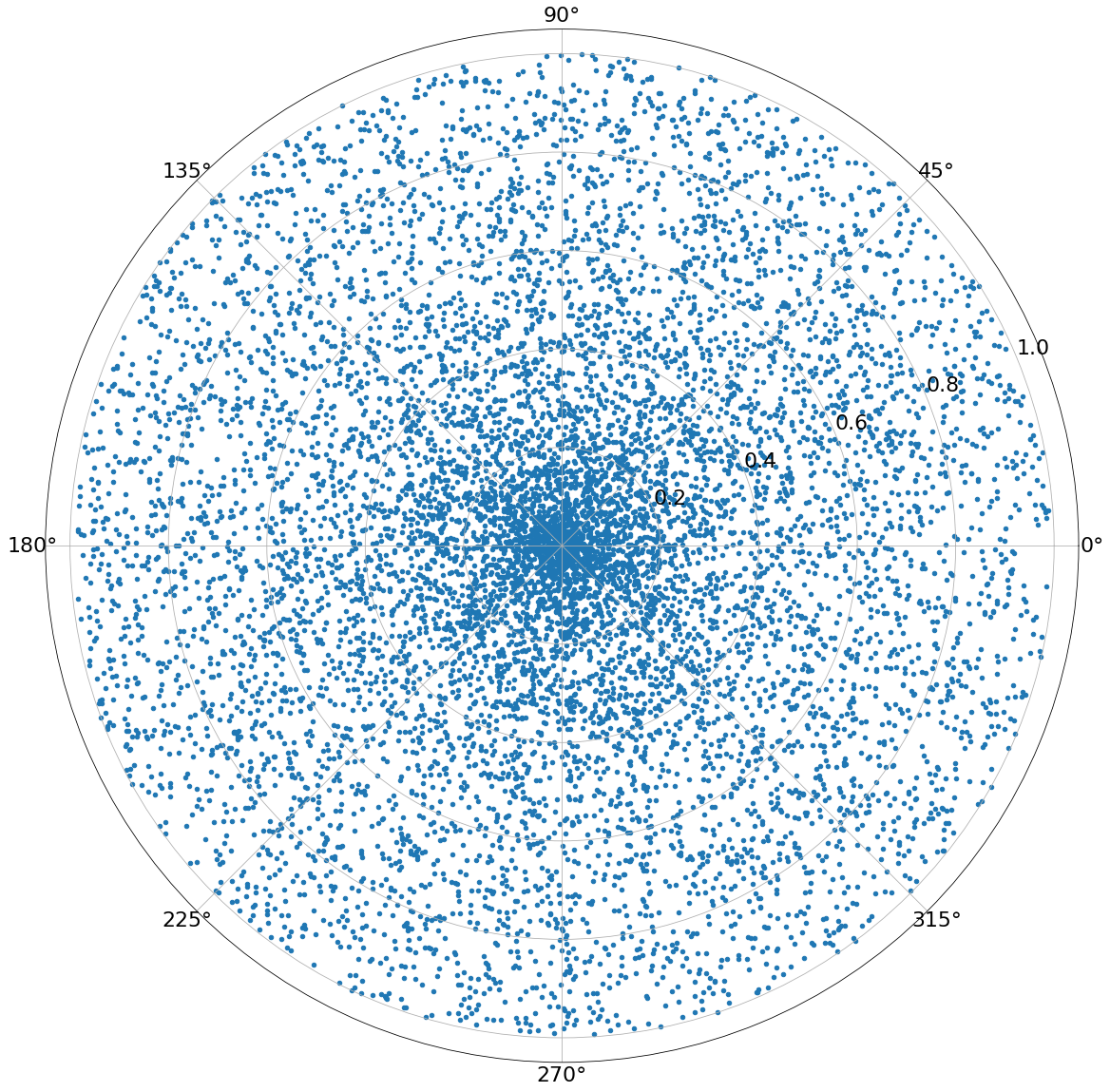
Uniform Disc
One way to sample points in a disc is to generate a random number between \(0\) and \(r\) for the radius and another one for the angle in \([0,2]\). The points won’t be uniformly distributed like that, since the area of segments on the inside is different from that of the outside. The sampling will look something like this:
np.random.seed(19680801)

N2 = 10000
R = 1
# radius in [0,R]
r = np.random.rand(N2) * R
# alpha in [0, 2pi]
alpha = np.random.rand(N2) * 2 * np.pi


fig = plt.figure()
ax = fig.add_subplot(projection='polar')
ax.scatter(alpha,r, s=20, alpha=1)
plt.show()
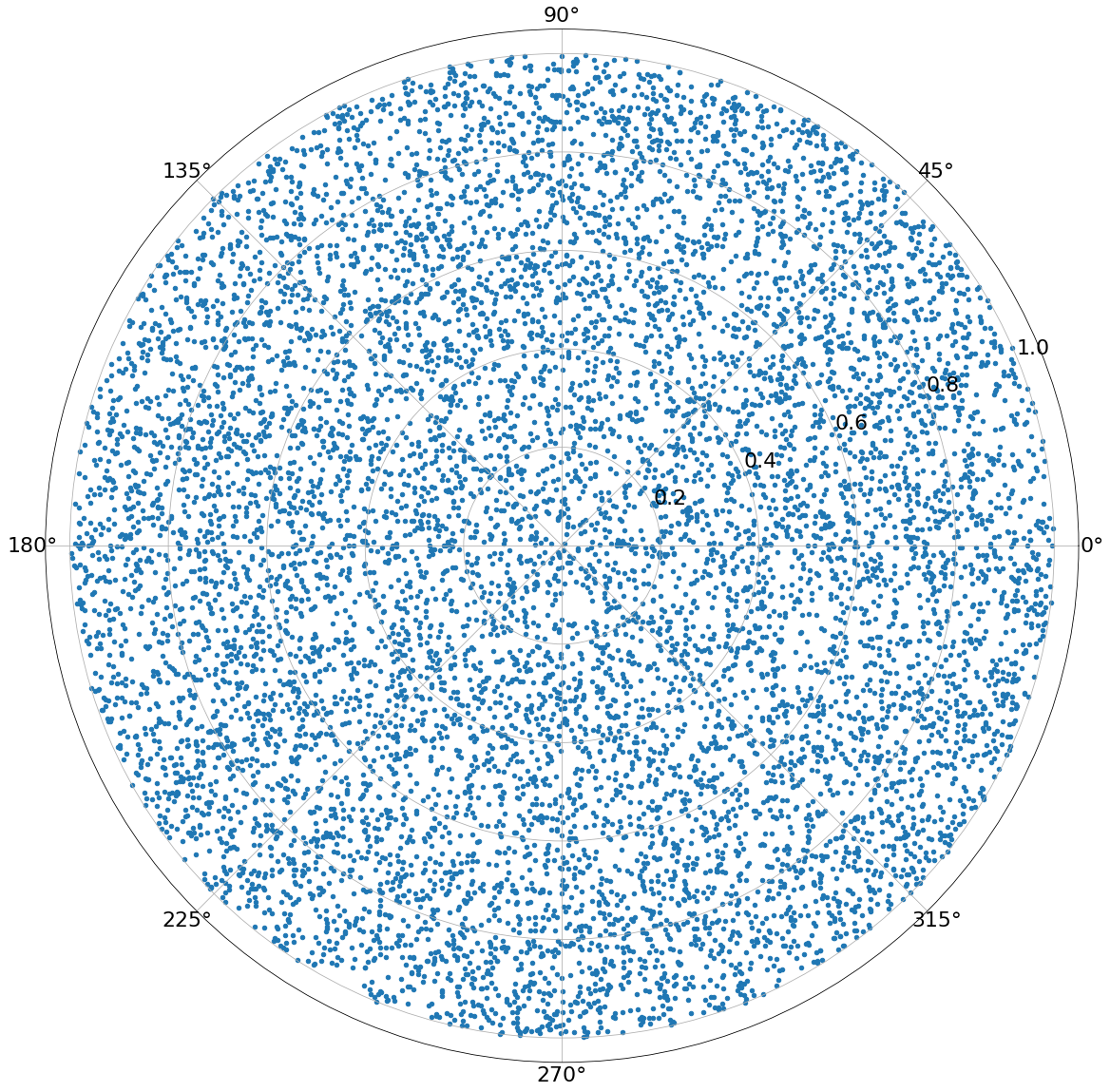
The points are focused in the center! With uniform area sampling it looks like the following:
u_1 = np.random.rand(N2)
u_2 = np.random.rand(N2)

r = np.sqrt(u_1) * R
alpha = u_2 * 2 * np.pi

fig = plt.figure()
ax = fig.add_subplot(projection='polar')
ax.scatter(alpha,r,s=20,alpha=1)
plt.show()
Algorithm:
Generate points uniformly distributed over the area of a disk with radius \(R\)
- Choose uniform numbers \(u_1, u_2\) in \([0,1]\)
- Calculate \(r = \sqrt{u_1}R\)
- Calculate \(\alpha = 2\pi u_2\)
Optionally convert to cartesian coordinates with:
\[x=r\cos\alpha\] \[y=r\sin\alpha\]PDF Used In Monte Carlo Integration
\[p(\alpha)= \frac{1}{\pi R^2}\] \[p(r,\alpha) = \frac{r}{\pi R^2}\]Derivation:
We want our distribution to be uniform in area over the disk. We will therefore integrate over the entire area \(A\).
The probability distribution function (pdf) has to integrate to \(1\) over the complete region. Since we want it to be uniform, it will just be some constant for each area element => \(p(a)=c\)
\[\int_{A}p(a)da = \int_{A}cda = c \int_{A}da = 1\]The easy way:
We know that the area of a disc is \(\pi R^2\).
\[c \int_{A}da = 1 \Rightarrow c\pi R^2 = 1 \Rightarrow c = \frac{1}{\pi R^2}\]The complicated way:
An area element \(da\) can be decomposed as \(da=dxdy\) (the very small area is just a rectangle). We then define a mapping from polar to cartesian coordinates:
\[x = r\cos\alpha = f_x(r, \alpha)\frac{\partial f_x(r, \alpha)}{\partial r}\] \[y = r\sin\alpha = f_y(r, \alpha)\]To do a coordinate transformation we have to find the determinant of the Jacobian of this transformation.
\[\begin{aligned} J &= \begin{pmatrix} \frac{\partial f_x(r, \alpha)}{\partial r}& \frac{\partial f_x(r, \alpha)}{\partial \alpha} \\ \frac{\partial f_y(r, \alpha)}{\partial r} & \frac{\partial f_y(r, \alpha)}{\partial \alpha} \end{pmatrix} \\ &= \begin{pmatrix} \cos\alpha & -r\sin\alpha \\ \sin\alpha & r\cos\alpha \end{pmatrix} \end{aligned}\]The determinant is thus:
\[\det{J} = r\cos\alpha \cos\alpha - (-r\sin\alpha \sin\alpha) = r\cos^2\alpha + r\sin^2\alpha = r(\cos^2\alpha + \sin^2\alpha) = r\]Computing the integral from before:
\[\begin{aligned} c \int_{A}da &= c \int_{A}dxdy \\ &= c \int_0^{R}\int_0^{2\pi} rdrd\alpha \\ &= c \int_0^{R}rdr\int_0^{2\pi} d\alpha \\ &= c \int_0^{R}rdr [\alpha]_0^{2\pi} \\ &= c \int_0^{R}rdr \\ &= 2 c \pi \int_0^{R}rdr \\ &= 2 c \pi [\frac{r^2}{2}]_0^R \\ &= c\pi R^2 \end{aligned}\]Setting this result equal to \(1\) and solving for \(c\) will give the desired result
Marginal And Conditional Densities:
We have \(p(a)=\frac{1}{\pi R^2}\). With the transformation from the last step we get \(p(r,\alpha)=\frac{r}{\pi R^2}\) (Transform into polar angles by adding the factor \(r\))
First the marginal density:
\[\begin{aligned} p_r(r) &= \int_0^{2\pi} p(r,\alpha)d\alpha\\ &= \int_0^{2\pi} \frac{r}{\pi R^2}d\alpha \\ &= \frac{r}{\pi R^2}\int_0^{2\pi} d\alpha \\ &= \frac{r}{\pi R^2} 2\pi \\ &= \frac{2r}{R^2} \end{aligned}\]The conditional probability:
\[p(\alpha \vert r) = \frac{p(r,\alpha)}{p_r(r)} = \frac{rR^2}{\pi R^2 2r} = \frac{1}{2\pi}\]Compute CDFs
\[P_r(r) = \int_0^r p_r(r')dr' = \int_0^r \frac{2r'}{R^2}dr' = \frac{2}{R^2}[\frac{r^2}{2}]_0^r = \frac{r^2}{R^2}\] \[P(\alpha \vert r) = \int_0^\alpha p(\alpha' \vert r)d\alpha' = \int_0^\alpha \frac{1}{2\pi}d\alpha' = \frac{\alpha}{2\pi}\]Invert CDFs
\[\begin{aligned} u_1 &= P_r(r) \\ &= \frac{r^2}{R^2} \\ u_1 R^2 &= r^2 \\ \sqrt{u_1R^2} &= r \\ \sqrt{u_1}R &= r \end{aligned}\] \[\begin{aligned} u_2 &= P(\alpha \vert r) \\ &= \frac{\alpha}{2\pi} \\ 2\pi u_2 &= \alpha \end{aligned}\]Sampling Hemisphere Directions
The following sections cover different related methods to sample (weighted) hemisphere regions.
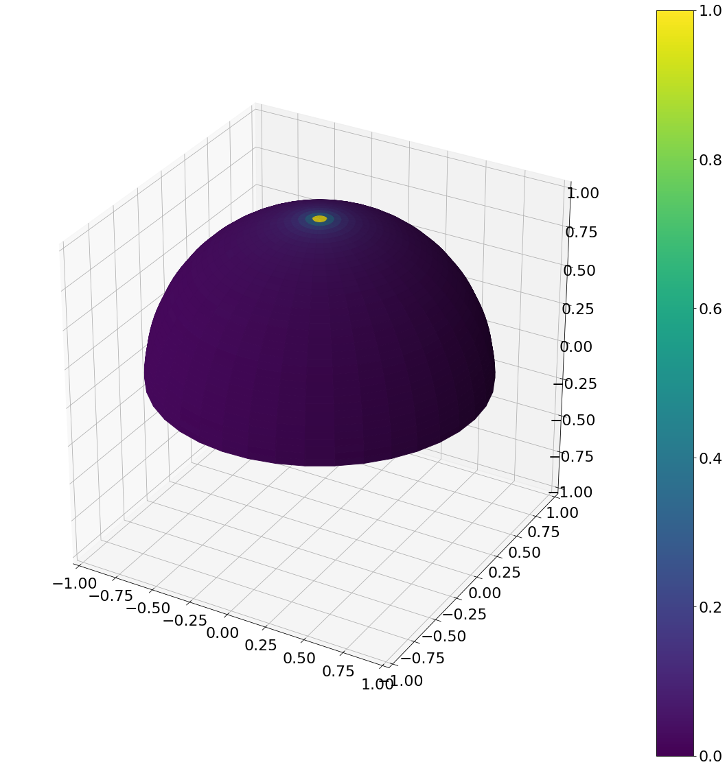
Uniform Unit Hemisphere
Sampling of points uniformly on the hemisphere. As with the disk, just randomly choosing two angles won’t give the desired result
u_1 = np.random.rand(N)
u_2 = np.random.rand(N)

# spherical angles

theta = u_1 * np.pi / 2
phi = u_2 * 2 * np.pi

hemisphereheatmap(theta,phi,hemi_res)
plt.show()
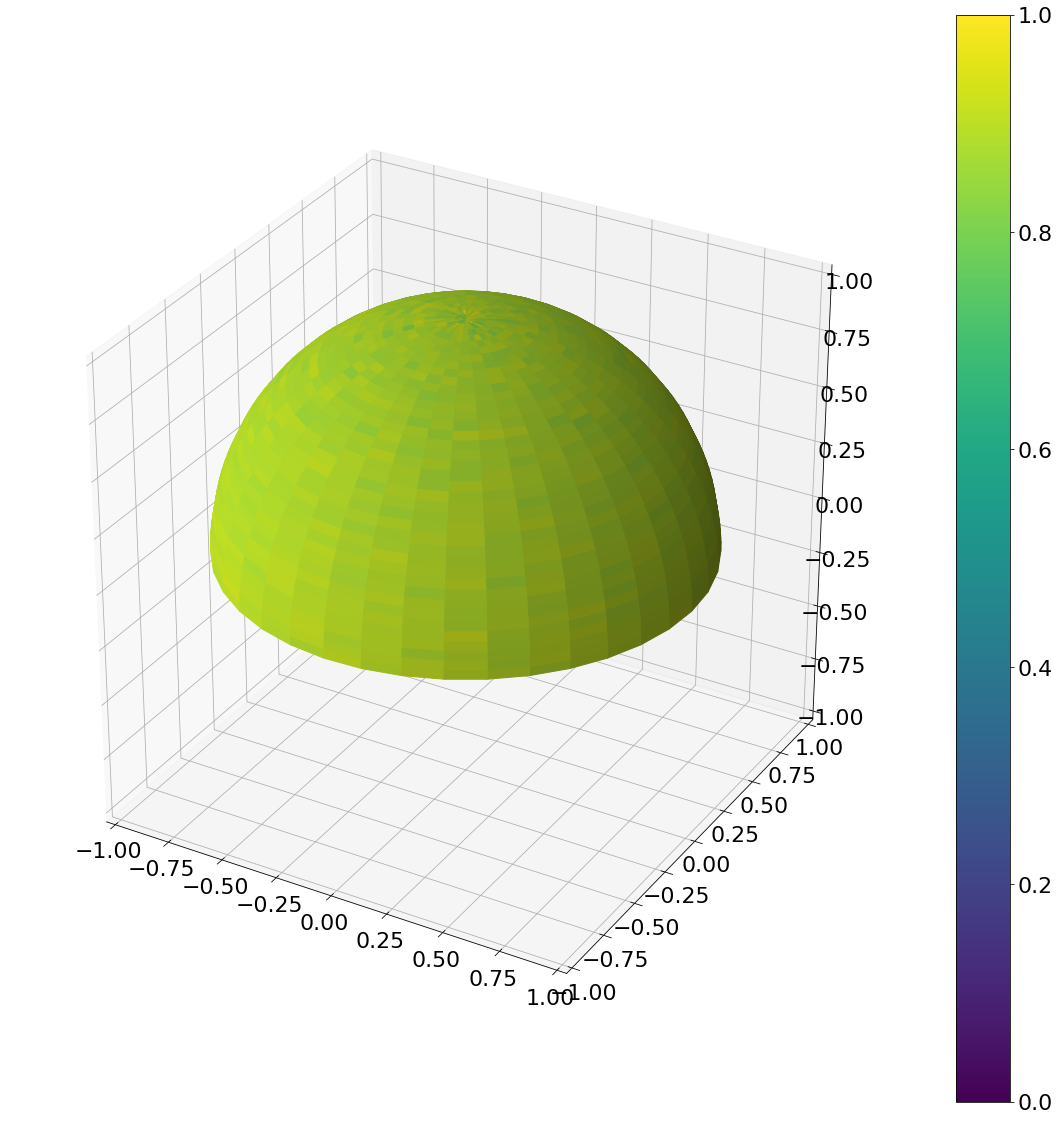
Now the result with a uniform area sampling of the upper hemisphere
def uniform_hemisphere(N):
    u_1 = np.random.rand(N)
    u_2 = np.random.rand(N)
    theta = np.arccos(1 - u_1)
    phi = u_2 * 2 * np.pi

    return theta, phi
theta, phi = uniform_hemisphere(N)

hemisphereheatmap(theta,phi,hemi_res)
plt.show()
Algorithm
Generate uniform points on the hemisphere
- Choose uniform numbers \(u_1, u_2\) in \([0,1]\)
- Calculate \(\theta = \cos^{-1}(1-u_1)\) or \(\theta = \cos^{-1}(u_1)\)
- Calculate \(\phi = 2\pi u_2\)
Optionally convert to cartesian coordinates with:
\[x = \sin\theta\cos\phi\] \[y = \sin\theta\sin\phi\] \[z = \cos\theta\]PDF Used In Monte Carlo Integration
\[p(\omega) = \frac{1}{2\pi}\] \[p(\theta, \phi) = \frac{1}{2\pi}\sin\theta\]Derivation
This is a special case of the general form discussed in the next section, but is shown as an example in more detail.
We want the pdf to be uniform over the unit hemisphere, so it will just be some constant for each solid angle \(\Rightarrow p(\omega) = c\)
\[\int_\Omega p(\omega)d\omega = \int_\Omega c d\omega = c \int_\Omega d\omega = 1\]The easy way:
We know that the solid angle of the hemisphere is \(2\pi\) . In general, for uniform sampling the pdf is just \(\frac{1}{\operatorname{Vol}(\Omega)}\) , where \(\operatorname{Vol}\) is the volume of the sample space.
\[c\int_\Omega d\omega \Rightarrow c2\pi = 1 \Rightarrow c = \frac{1}{2\pi}\]The complicated way:
\[\begin{aligned} \int_\Omega p(\omega)d\omega &= \int_0^{\frac{\pi}{2}}\int_0^{2\pi}c\sin\theta d\theta d\phi \\ &= c 2\pi \int_0^{\frac{\pi}{2}}\sin\theta d\theta \\ &= c2\pi [-\cos\theta]_0^{\frac{\pi}{2}} \\ &= c2\pi (\cos 0 - \cos\frac{\pi}{2}) \\ &= c2\pi \end{aligned}\]Therefore \(c2\pi = 1 \Rightarrow c = \frac{1}{2\pi}\)
To convert to the angular representation, we have to add (The factor can be found similarly to the \(r\) factor of the disk)
\[p(\omega) = p(\theta,\phi)\sin\theta\]Marginal And Conditional Densities:
\[p_\theta(\theta) = \int_0^{2\pi} p(\theta,\phi)\sin\theta d\phi = \int_0^{2\pi}\frac{1}{2\pi}\sin\theta d\phi = \frac{1}{2\pi}\sin\theta * 2\pi = \sin\theta\] \[p(\phi \vert \theta) = \frac{p(\theta,\phi)}{p_\theta(\theta)} = \frac{\sin\theta}{2\pi\sin\theta} = \frac{1}{2\pi}\]Compute CDFs
\[P_\theta(\theta) = \int_0^\theta \sin\theta' d\theta' = [-\cos(\theta')]_0^\theta = \cos 0 - \cos\theta = 1 - \cos\theta\] \[P(\phi \vert \theta) = \int_0^\phi p(\phi' \vert \theta)d\phi' = \int_0^\phi \frac{1}{2\pi}d\phi' = \frac{\phi}{2\pi}\]Invert CDFs
\[u_1 = P_\theta(\theta) = 1 - \cos\theta \Rightarrow \cos\theta = 1 - u_1 \Rightarrow \theta = \cos^{-1}(1- u_1)\] \[u_2 = P(\phi \vert \theta) = \frac{\phi}{\theta} \Rightarrow 2\pi u_2 = \phi\]Power Cosine Weighted Hemisphere Sector
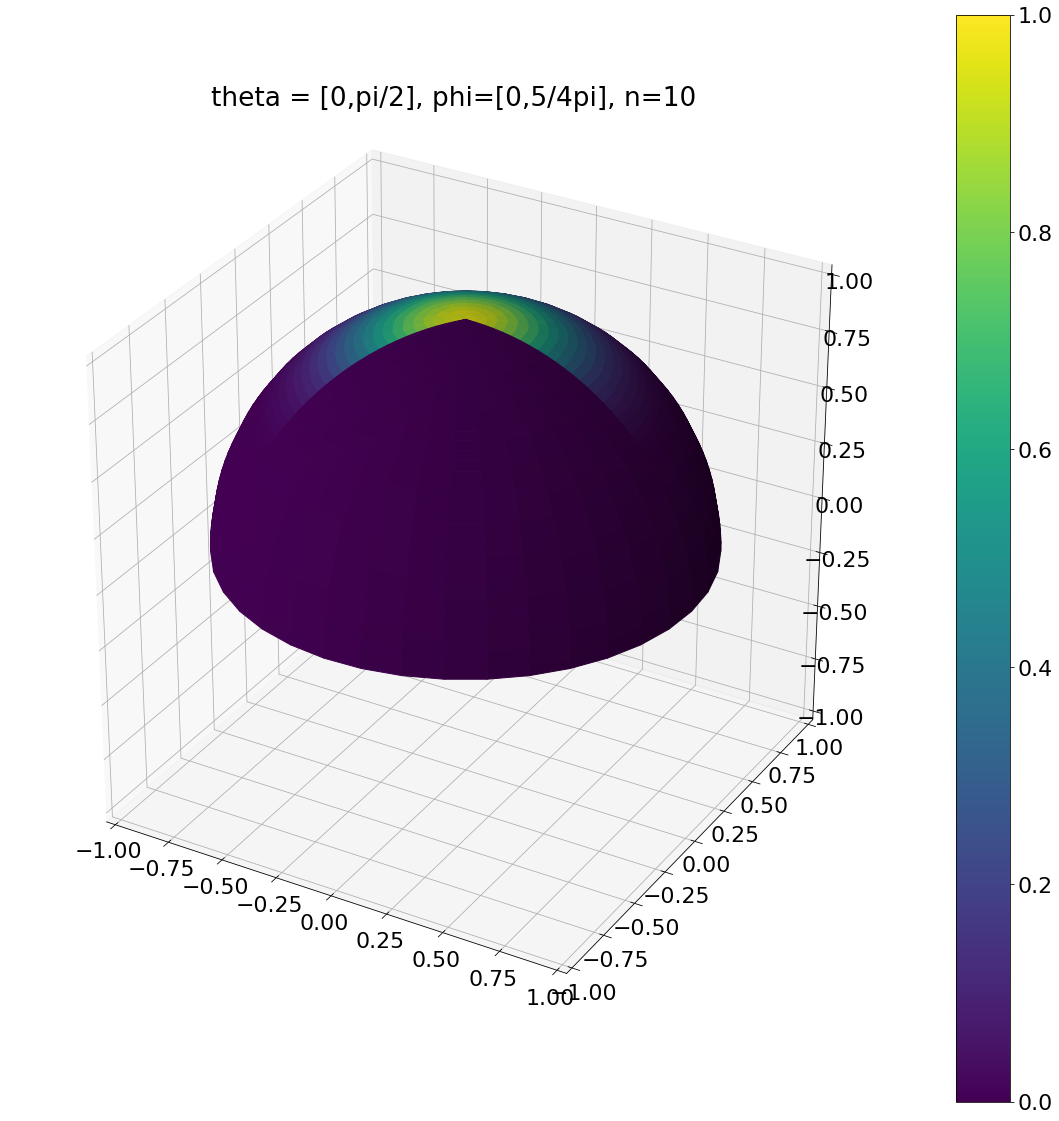
The following distrbution is chosen, since it includes some other cases (uniform cap, uniform hemisphere, cosine weighted hemisphere, …). Can be used to account for the \(\cos\) factor in the rendering equation or for something like the phong model.
The probability of each sample is weighted by its cosine with the normal. Samples are chosen from only a part of the hemisphere, defined by minimum and maximum angles.
Here are some examples:
def pow_cos_hemisphere_sector(theta_min,theta_max,phi_min,phi_max,n,N):
    u_1 = np.random.rand(N)
    u_2 = np.random.rand(N)

    theta = np.arccos(np.power(
        math.pow(math.cos(theta_min),n+1) - u_1*(math.pow(math.cos(theta_min),n+1) - math.pow(math.cos(theta_max),n+1))
        ,1/(n+1)))
    phi = u_2*(phi_max - phi_min)

    return theta,phi
# spherical angles
theta, phi = pow_cos_hemisphere_sector(0,np.pi/2,0,np.pi*5/4,10,N)
ax = hemisphereheatmap(theta,phi,hemi_res)
ax.set_title("theta = [0,pi/2], phi=[0,5/4pi], n=10")
plt.show()
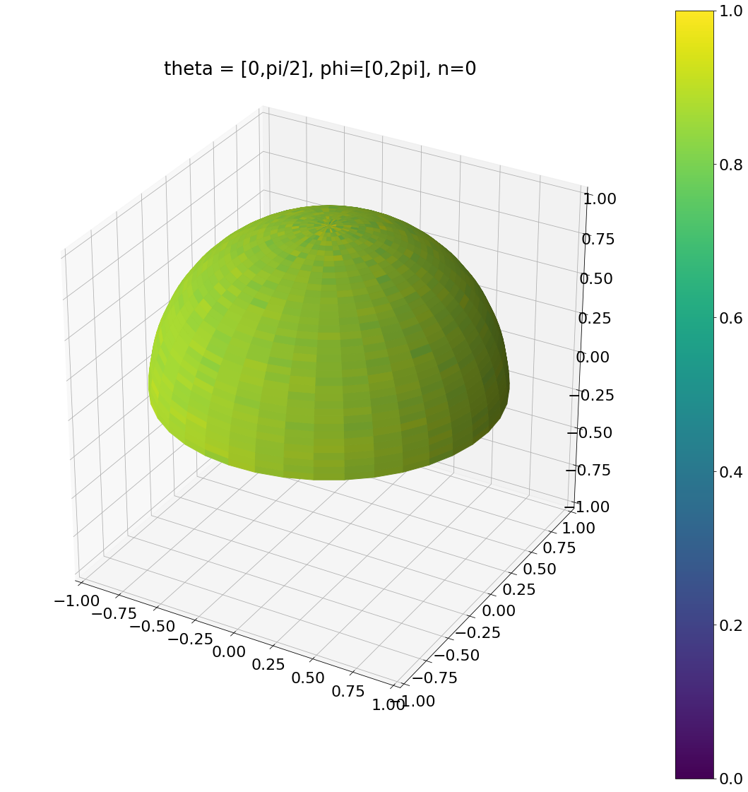
theta, phi = pow_cos_hemisphere_sector(0,np.pi/2,0,np.pi*2,0,N)
ax = hemisphereheatmap(theta,phi,hemi_res)
ax.set_title("theta = [0,pi/2], phi=[0,2pi], n=0")
plt.show()
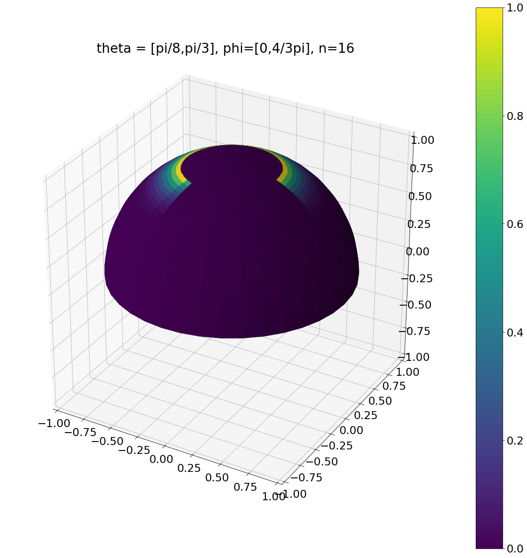
theta, phi = pow_cos_hemisphere_sector(np.pi/8,np.pi/3,0,np.pi*4/3,16,N)
ax = hemisphereheatmap(theta,phi,hemi_res)
ax.set_title("theta = [pi/8,pi/3], phi=[0,4/3pi], n=16")
plt.show()
Algorithm
Generate points weighted by a power cosine with power \(n\) on the sphere sector defined by the angles \(\theta_{min}, \theta_{max}, \phi_{min}, \phi_{max}\)
- Choose uniform numbers \(u_1, u_2\) in \([0,1]\)
- Calculate \(\theta = \cos^{-1}(\sqrt[n+1]{\cos^{n+1}\theta_{min} - u_1(cos^{n+1}\theta_{min} - \cos^{n+1}\theta_{max})} )\)
- Calculate \(\phi = u_2(\phi_{max} - \phi_{min})\)
Optionally convert to cartesian coordinates with:
\[x = \sin\theta\cos\phi\] \[y = \sin\theta\sin\phi\] \[z = \cos\theta\]PDF Used In Monte Carlo Integration
\[p(\omega) = \frac{n+1}{(\cos^{n+1}\theta_{min} - \cos^{n+1}\theta_{max})({\phi_{max}} - {\phi_{min}}) }\cos^n\theta\] \[p(\theta,\phi) = \frac{n+1}{(\cos^{n+1}\theta_{min} - \cos^{n+1}\theta_{max})({\phi_{max}} - {\phi_{min}})}\cos^n\theta\sin\theta\]Derivation
Each direction should be weighted by a power \(n\) of the cosine of the direction’s polar angle, therefore it is proportional to \(\cos^n\theta \Rightarrow p(\omega) = c\cos^n\theta\)
\[\int_{\Omega_r} p(\omega)d\omega = \int_{\Omega_r} c \cos^n\theta d\omega = c\int_{\Omega_r} \cos^n\theta d\omega = 1\]Here \(\Omega_r\) is the ring of the sphere, which is specified by a minimum and maximum angles \(\theta_{min}, \theta_{max}, \phi_{min}, \phi_{max}\)
Normalization factor
\[c\int_{\Omega_r} \cos^n\theta d\omega = c\int_{\theta_{min}}^{\theta_{max}}\int_{\phi_{min}}^{\phi_{max}} \cos^n\theta\sin\theta d\theta d\phi = c({\phi_{max}} - {\phi_{min}})\int_{\theta_{min}}^{\theta_{max}}\cos^n\theta\sin\theta d\theta\]We evaluate the integral on the right using partial integration and denoting the integral itself as \(I\)
\[\begin{aligned} I &= \int_{\theta_{min}}^{\theta_{max}}\cos^n\theta\sin\theta d\theta \\ &= [\cos^n\theta (-\cos\theta)]_{\theta_{min}}^{\theta_{max}} - \int_{\theta_{min}}^{\theta_{max}}-n\cos^{n-1}\theta\sin\theta (-\cos\theta)d\theta \\ &= [-\cos^{n+1}\theta]_{\theta_{min}}^{\theta_{max}} -n\int_{\theta_{min}}^{\theta_{max}}\cos^n\sin\theta d\theta \\ &= \cos^{n+1}\theta_{min} - \cos^{n+1}\theta_{max} - nI \\ I + nI &= \cos^{n+1}\theta_{min} - \cos^{n+1}\theta_{max} \\ I &= \frac{\cos^{n+1}\theta_{min} - \cos^{n+1}\theta_{max}}{n+1} \\ I &= \frac{d}{n+1} \end{aligned}\]In the last line, we just introduced a new variable to make writing easier.
Putting this in the first equation:
\[c({\phi_{max}} - {\phi_{min}})\int_{\theta_{min}}^{\theta_{max}} \cos^n\theta\sin\theta d\theta = c({\phi_{max}} - {\phi_{min}})\frac{d}{n+1} = 1 \Rightarrow c = \frac{n+1}{d({\phi_{max}} - {\phi_{min}})}\]This results in:
\[p(\omega) = \frac{n+1}{d({\phi_{max}} - {\phi_{min}}) }\cos^n\theta \Rightarrow p(\theta,\phi) = \frac{n+1}{d({\phi_{max}} - {\phi_{min}})}\cos^n\theta\sin\theta\]Marginal And Conditional Densities:
\[p_\theta(\theta) = \int_{\phi_{min}}^{\phi_{max}}p(\theta,\phi) d\phi = \int_{\phi_{min}}^{\phi_{max}}\frac{n+1}{d({\phi_{max}} - {\phi_{min}})}\cos^n\theta\sin\theta d\phi = \frac{n+1}{d({\phi_{max}} - {\phi_{min}})}\cos^n\theta\sin\theta ({\phi_{max}} - {\phi_{min}}) = \frac{n+1}{d}\cos^n\theta\sin\theta\] \[p(\phi \vert \theta) = \frac{p(\theta,\phi)}{p_\theta(\theta)} = \frac{(n+1)\cos^n\theta\sin\theta d}{d({\phi_{max}} - {\phi_{min}}) (n+1)\cos^n\theta\sin\theta}= \frac{1}{\phi_{max} - \phi_{min} }\]Compute CDFs
\[P_\theta(\theta) = \int_{\theta_{min}}^{\theta}\frac{n+1}{d}\cos^n\theta'\sin\theta'd\theta' = \frac{n+1}{d}\int_{\theta_{min}}^{\theta}\cos^n\theta'\sin\theta'd\theta'\]We already integrated the integral expression before, so we can use that
\[\frac{n+1}{d}\int_{\theta_{min}}^{\theta}\cos^n\theta'\sin\theta'd\theta' = \frac{n+1}{d}\frac{\cos^{n+1}\theta_{min} - \cos^{n+1}\theta}{n+1} = \frac{\cos^{n+1}\theta_{min} - \cos^{n+1}\theta}{\cos^{n+1}\theta_{min} - \cos^{n+1}\theta_{max}}\] \[P(\phi \vert \theta) = \int_{\phi_{min}}^{\phi}p(\phi ' \vert \theta)d\phi' = \int_{\phi_{min}}^{\phi} \frac{1}{\phi_{max} - \phi_{min} }d\phi' =\frac{\phi}{\phi_{max} - \phi_{min}}\]Invert CDFs
\[\begin{aligned} u_1 &= P_\theta(\theta)\\ &= \frac{\cos^{n+1}\theta_{min} - \cos^{n+1}\theta}{\cos^{n+1}\theta_{min} - \cos^{n+1}\theta_{max}} \\ u_1(cos^{n+1}\theta_{min} - \cos^{n+1}\theta_{max}) &= \cos^{n+1}\theta_{min} - \cos^{n+1}\theta \\ \cos^{n+1}\theta &= \cos^{n+1}\theta_{min} - u_1(cos^{n+1}\theta_{min} - \cos^{n+1}\theta_{max}) \\ \cos\theta &= \sqrt[n+1]{\cos^{n+1}\theta_{min} - u_1(cos^{n+1}\theta_{min} - \cos^{n+1}\theta_{max})} \\ \theta &= \cos^{-1}(\sqrt[n+1]{\cos^{n+1}\theta_{min} - u_1(cos^{n+1}\theta_{min} - \cos^{n+1}\theta_{max})} ) \end{aligned}\] \[\begin{aligned} u_2 &= P(\phi \vert \theta) \\ &= \frac{\phi}{\phi_{max} - \phi_{min}}\\ \phi &= u_2(\phi_{max} - \phi_{min}) \end{aligned}\]Power Cosine Weighted Hemisphere Cap
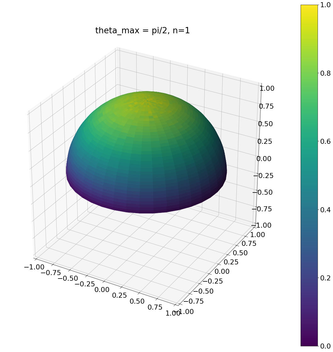
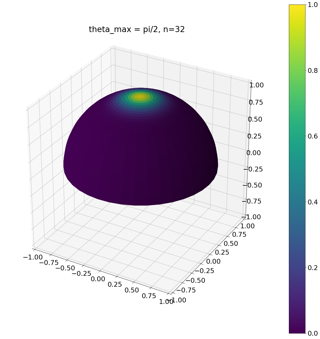
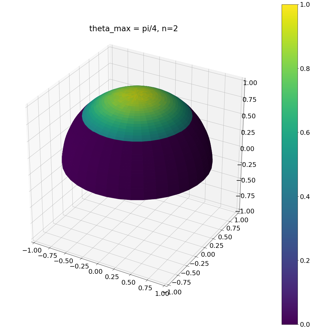
The probability of each sample is weighted by a power of its cosine with the normal. Samples are chosen from a cap of the hemisphere, defined by a maximum elevation angle.
Here are some examples:
def pow_cos_hemisphere_cap(theta_max,n,N):
    u_1 = np.random.rand(N)
    u_2 = np.random.rand(N)

    theta = np.arccos(np.power(
        1 - u_1*(1- math.pow(math.cos(theta_max),n+1))
        ,1/(n+1)))
    phi = u_2*np.pi*2

    return theta,phi
theta, phi = pow_cos_hemisphere_cap(np.pi/2,1,N)
ax = hemisphereheatmap(theta,phi,hemi_res)
ax.set_title("theta_max = pi/2, n=1")
plt.show()

theta, phi = pow_cos_hemisphere_cap(np.pi/2,32,N)
ax = hemisphereheatmap(theta,phi,hemi_res)
ax.set_title("theta_max = pi/2, n=32")
plt.show()

theta, phi = pow_cos_hemisphere_cap(np.pi/4,2,N)
ax = hemisphereheatmap(theta,phi,hemi_res)
ax.set_title("theta_max = pi/4, n=2")
plt.show()
Algorithm
Generate points weighted by a power cosine with power \(n\) on the sphere cap defined by the maximum elevation angle \(\theta_{max}\)
- Choose uniform numbers \(u_1, u_2\) in \([0,1]\)
- Calculate \(\theta = \cos^{-1}(\sqrt[n+1]{1 - u_1(1- \cos^{n+1}\theta_{max})} )\)
- Calculate \(\phi = 2\pi u_2\)
Optionally convert to cartesian coordinates with:
\[x = \sin\theta\cos\phi\] \[y = \sin\theta\sin\phi\] \[z = \cos\theta\]PDF Used In Monte Carlo Integration
\[p(\omega) = \frac{n+1}{2\pi(1 - \cos^{n+1}\theta_{max}) }\cos^n\theta\] \[p(\theta,\phi) = \frac{n+1}{2\pi(1 - \cos^{n+1}\theta_{max}) }\cos^n\theta\sin\theta\]Derivation
This is a special case of the power cosine weighted hemisphere sector with \(\phi_{min}=0, \phi_{max}=2\pi, \theta_{min} = 0\)
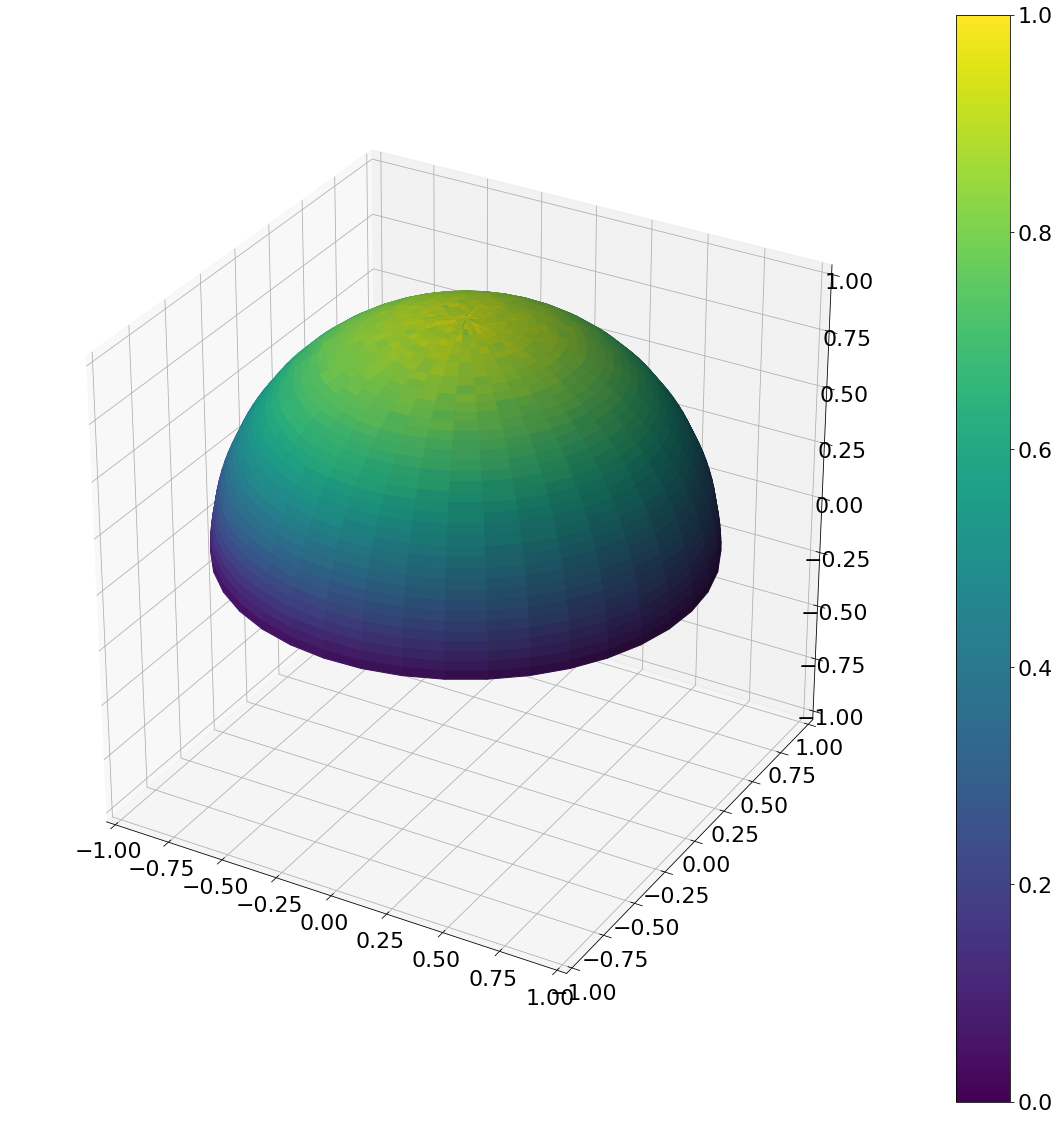
Cosine Weighted Hemisphere
The probability of each sample is weighted by its cosine with the normal.
Here is the result:
def cos_hemisphere(N):
    u_1 = np.random.rand(N)
    u_2 = np.random.rand(N)

    theta = np.arccos(np.sqrt(1 - u_1))
    phi = u_2*np.pi*2

    return theta,phi
theta, phi = cos_hemisphere(N)

ax = hemisphereheatmap(theta,phi,hemi_res)
plt.show()
Algorithm
Generate points weighted by the cosine hemisphere.
- Choose uniform numbers \(u_1, u_2\) in \([0,1]\)
- Calculate \(\theta = \cos^{-1}(\sqrt{1 - u_1} )\)
- Calculate \(\phi = 2\pi u_2\)
Optionally convert to cartesian coordinates with:
\[x = \sin\theta\cos\phi\] \[y = \sin\theta\sin\phi\] \[z = \cos\theta\]PDF Used In Monte Carlo Integration
\[p(\omega) = \frac{1}{\pi}\cos\theta\] \[p(\theta,\phi) = \frac{1}{\pi}\cos\theta\sin\theta\]Derivation
This is a special case of the power cosine weighted hemisphere cap with \(\theta_{max} = \frac{\pi}{2}, n = 1\)
Sampling Distribution Of Normals
The following algorithms and derivations are for the three commonly used distribution of normal functions for microfacet BRDFs: Beckmann, Phong and Trowbridge–Reitz/GGX.
Note, that all the sampling algorithms are for the microfacet normal, which is used to reflect the incoming ray to get the outgoing direction. Because of that, all probabilities have to be scaled by \(\frac{1}{4\omega_o \cdot \omega_h} = \frac{1}{4\omega_i \cdot \omega_h}\) to account for the change of measure between the sampled normal (half vector) and incoming direction.
I used the distribution formulas given in Walter et al. (Microfacet Models for Refraction through Rough Surfaces), though I did change the notation a bit to make it easier to write. Hopefully there won’t be any confusion. The characteristic functions for the hemisphere check are not included, as they are not that relevant for the sampling, though you should be careful to include them in an implementation that needs to compute the probability densities for arbitrary directions.
Note, that these distributions of normales are normalized, such that:
\[\int_\Omega \operatorname{D}(\omega)\cos\theta d\omega= 1\]This means, the PDF is \(\operatorname{D}(\omega)\cos\theta\)
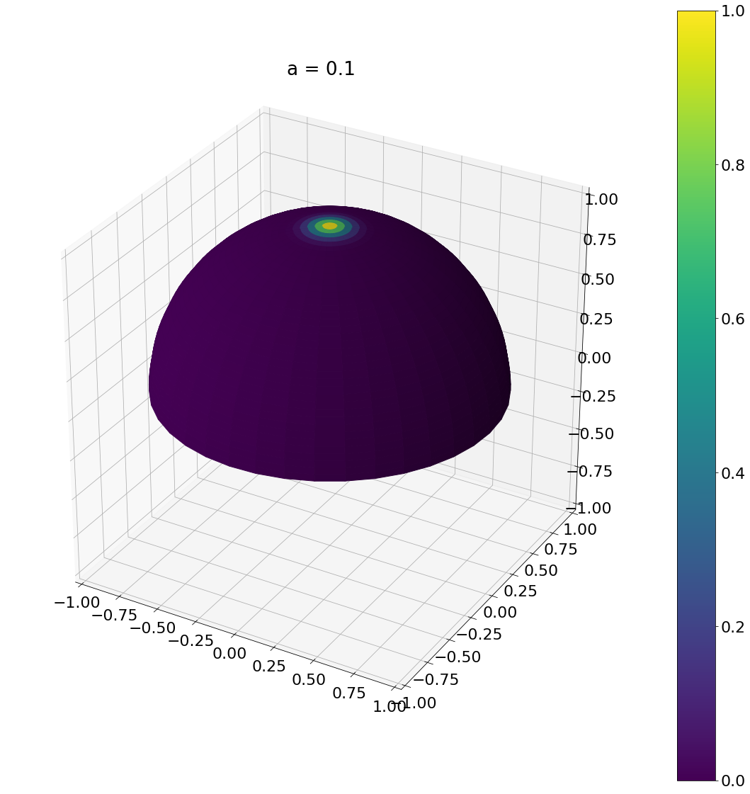
Beckmann Distribution
The normals of the microfacets are distributed according to the Beckmann distribution:
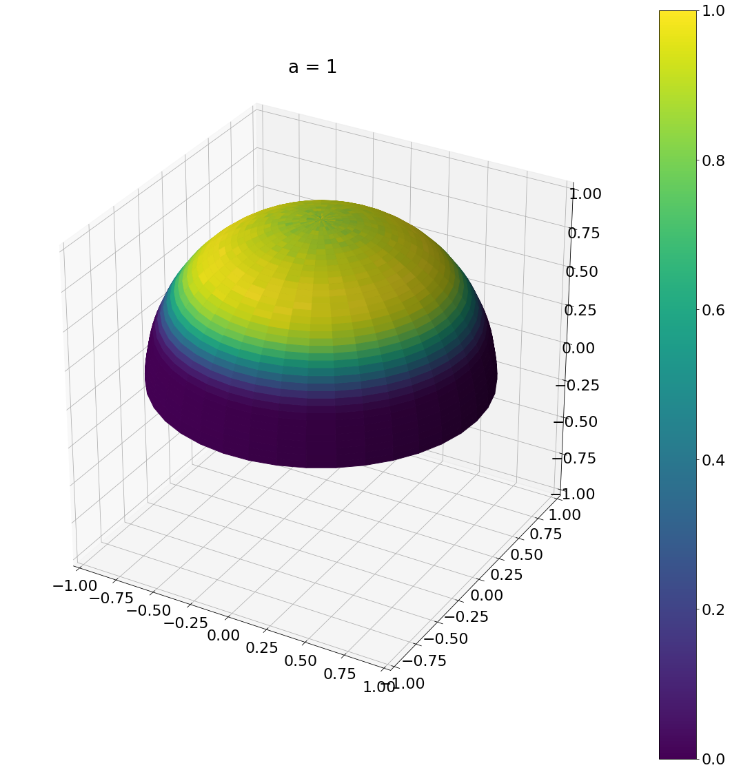
\[\begin{aligned} \operatorname{D}(\omega) &= \frac{1}{\pi a_b^2\cos^4\theta}\exp{\frac{-\tan^{2}\theta}{a_b^2}}\\ \operatorname{D}(\theta,\phi) &= \frac{\sin\theta}{\pi a_b^2\cos^4\theta}\exp{\frac{-\tan^{2}\theta}{a_b^2}} \end{aligned}\]Here is the result:
def sample_beckmann(a,N):
    u_1 = np.random.rand(N)
    u_2 = np.random.rand(N)

    theta = np.arctan(np.sqrt(-a*a*np.log(1 - u_1)))
    phi = u_2*np.pi*2

    return theta,phi
theta, phi = sample_beckmann(0.1,N)
ax = hemisphereheatmap(theta,phi,hemi_res)
ax.set_title("a = 0.1")

plt.show()

theta, phi = sample_beckmann(0.5,N)
ax = hemisphereheatmap(theta,phi,hemi_res)
ax.set_title("a = 0.5")

plt.show()

theta, phi = sample_beckmann(1,N)
ax = hemisphereheatmap(theta,phi,hemi_res)
ax.set_title("a = 1")
plt.show()

Algorithm
Sample microfacet normal according to the Beckmann distribution:
- Choose uniform numbers \(u_1, u_2\) in \([0,1]\)
- Calculate \(\theta = \tan^{-1}( \sqrt{-a_b^2\log (1-u_1)})\) or \(\theta = \tan^{-1}( \sqrt{-a_b^2\log (u_1)})\)
- Calculate \(\phi = 2\pi u_2\)
Optionally convert to cartesian coordinates with:
\[x = \sin\theta\cos\phi\] \[y = \sin\theta\sin\phi\] \[z = \cos\theta\]PDF Used In Monte Carlo Integration
\[p_m(\omega) = \frac{\cos\theta}{\pi a_b^2\cos^4\theta}\exp{\frac{-\tan^{2}\theta}{a_b^2}} = \frac{1}{\pi a_b^2\cos^3\theta}\exp{\frac{-\tan^{2}\theta}{a_b^2}}\] \[p_m(\theta,\phi) = \frac{\cos\theta\sin\theta}{\pi a_b^2\cos^4\theta}\exp{\frac{-\tan^{2}\theta}{a_b^2}} = \frac{\tan\theta}{\pi a_b^2\cos^2\theta}\exp{\frac{-\tan^{2}\theta}{a_b^2}}\]Derivation
Due to normalization, the densities are given as follows:
\[\begin{aligned} p(\omega) &= D(\omega)\cos\theta\\ p(\theta,\phi) &= p(\omega)\sin\theta\\ &= \frac{\sin\theta\cos\theta}{\pi a_b^2\cos^4\theta}\exp{\frac{-\tan^{2}\theta}{a_b^2}} \\ &= \frac{\tan\theta}{\pi a_b^2\cos^2\theta}\exp{\frac{-\tan^{2}\theta}{a_b^2}} \end{aligned}\]Marginal And Conditional Densities:
\[\begin{aligned} p_\theta(\theta) &= \int_0^{2\pi}p(\theta,\phi)d\phi \\ &=\int_0^{2\pi}\frac{\tan\theta}{\pi a_b^2\cos^2\theta}\exp{\frac{-\tan^{2}\theta}{a_b^2}} d\phi \\ &= 2\pi\frac{\tan\theta}{\pi a_b^2\cos^2\theta}\exp{\frac{-\tan^{2}\theta}{a_b^2}} \\ &= 2\frac{\tan\theta}{ a_b^2\cos^2\theta}\exp{\frac{-\tan^{2}\theta}{a_b^2}} \\ &= 2\pi p(\theta, \phi) \end{aligned}\] \[p(\phi \vert \theta) = \frac{p(\theta,\phi)}{p_\theta(\theta)} = \frac{p(\theta,\phi)}{2\pi p(\theta,\phi)} = \frac{1}{2\pi}\]Compute CDFs
\[P_\theta(\theta) = \int_{0}^{\theta}2\frac{\tan\theta'}{ a_b^2\cos^2\theta'}\exp{\frac{-\tan^{2}\theta'}{a_b^2}}d\theta'\]To solve this integral, we change variables and introduce \(u = \tan\theta'\). That gives us \(du = (\tan\theta')'d\theta' = \frac{1}{\cos^2\theta'}d\theta'\). Solving for \(du\) (with the usual slight abuse of notation): \(d\theta' = \cos^2\theta' du\).
As we will resubstitute later, for now let’s disregard the limits:
\[\begin{aligned} P_\theta(\theta) &= \int 2\frac{\tan\theta'}{ a_b^2\cos^2\theta'}\exp{(\frac{-\tan^{2}\theta'}{a_b^2})} d\theta' \\ &= \frac{2}{a_b^2} \int \frac{u}{ \cos^2\theta'}\exp{(\frac{-u^{2}}{a_b^2})}\cos^2\theta' du\\ &= \frac{2}{a_b^2} \int u\exp{(\frac{-u^{2}}{a_b^2})} du \end{aligned}\]The integral can now be solved by basic means by considering the derivative of the exponential.
\[\begin{aligned} P_\theta(\theta) &= \frac{2}{a_b^2} \int u\exp{(\frac{-u^{2}}{a_b^2})} du\\ &= \frac{2}{a_b^2} [-\frac{1}{2}a_b^2\exp(\frac{-u^2}{a_b^2})] \\ &= -[\exp(\frac{-u^2}{a_b^2})] \end{aligned}\]Resubstituting \(u = \tan\theta'\):
\[\begin{aligned} P_\theta(\theta) &= \frac{2}{a_b^2} \int u\exp{(\frac{-u^{2}}{a_b^2})} du\\ &= -[\exp(\frac{-\tan^2\theta'}{a_b^2})]_0^{\theta}\\ &= -(\exp(\frac{-\tan^2\theta}{a_b^2}) - \exp(\frac{-\tan^20}{a_b^2}) ) \\ &= -(\exp(\frac{-\tan^2\theta}{a_b^2}) - 1 ) \\ &= 1- \exp(\frac{-\tan^2\theta}{a_b^2}) \end{aligned}\] \[P(\phi \vert \theta) = \int_{0}^{\phi}p(\phi ' \vert \theta)d\phi' = \int_{0}^{\phi} \frac{1}{2\pi }d\phi' =\frac{\phi}{2\pi}\]Invert CDFs
\[\begin{aligned} u_1 &= P_\theta(\theta)\\ &= 1- \exp(\frac{-\tan^2\theta}{a_b^2}) \\ u_1 - 1 &=- \exp(\frac{-\tan^2\theta}{a_b^2}) \\ 1- u_1 &= \exp(\frac{-\tan^2\theta}{a_b^2}) \\ \log (1-u_1) &= \frac{-\tan^2\theta}{a_b^2} \\ -a_b^2\log (1-u_1)&= \tan^2\theta \\ \sqrt{-a_b^2\log (1-u_1)}&= \tan\theta \\ \tan^{-1}( \sqrt{-a_b^2\log (1-u_1)}) &= \theta\\ \theta &=\tan^{-1}( \sqrt{-a_b^2\log (1-u_1)}) \end{aligned}\]Since \(u_1\) is uniformly distributed in \([0,1]\), so is \(1-u_1\), so we can use either of them for the generation.
\[\begin{aligned} u_2 &= P(\phi \vert \theta) \\ &= \frac{\phi}{2\pi}\\ \phi &= u_22\pi \end{aligned}\]Phong Distribution
The normals of the microfacets are distributed according to the Phong Distribution:
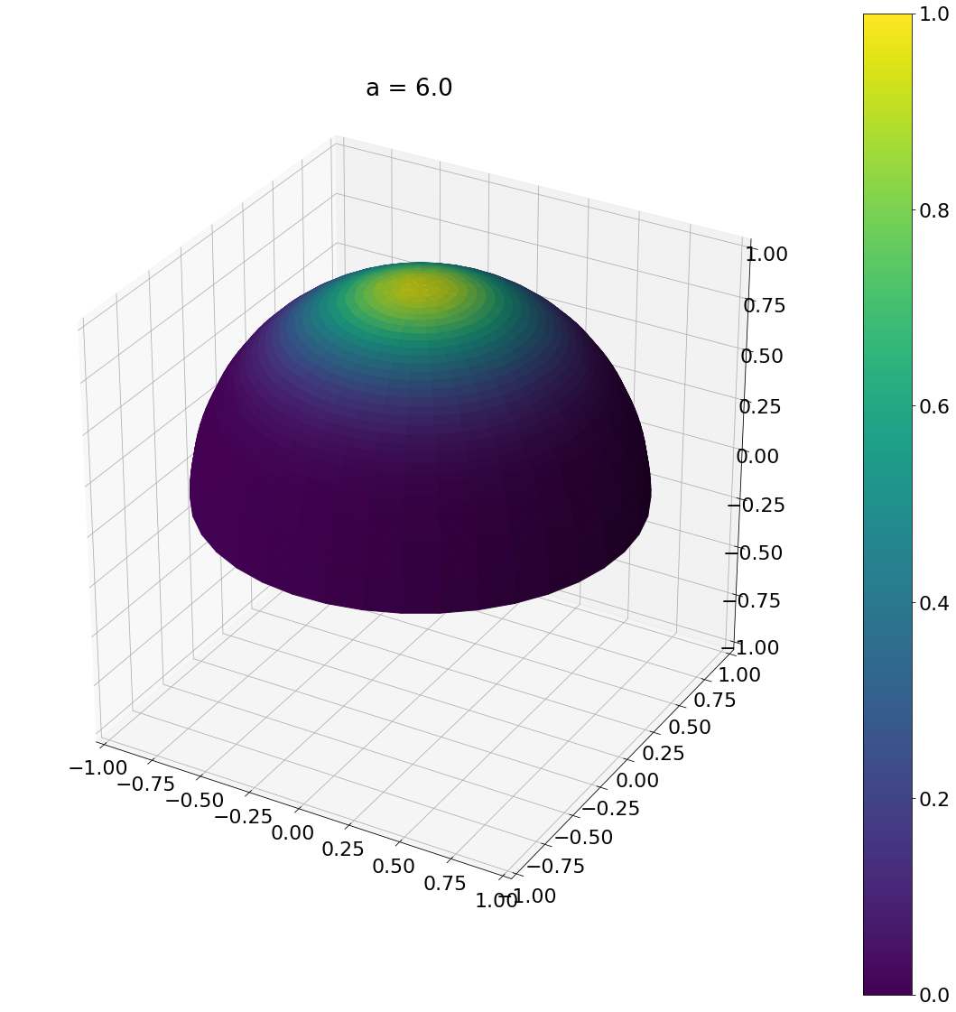
\[\begin{aligned} \operatorname{D}(\omega) &= \frac{a_p +2}{2\pi}\cos^{a_p}\theta\\ \operatorname{D}(\theta,\phi) &= \frac{a_p +2}{2\pi}\cos^{a_p}\theta\sin\theta \end{aligned}\]Walter et al. recommend a relation between the Beckmann \(a_b\) and the phong \(a_p\):
\[\begin{aligned} a_p &= 2a_b^{-2} - 2 \end{aligned}\]Here is the result:
def sample_phong_normal(a,N):
    return pow_cos_hemisphere_cap(np.pi/2,a+1,N)

def beckmann_width_to_phong(a):
    return 2/(a*a) - 2
a = beckmann_width_to_phong(0.1)
theta, phi = sample_phong_normal(a,N)
ax = hemisphereheatmap(theta,phi,hemi_res)
ax.set_title(f"a = {a}")
plt.show()
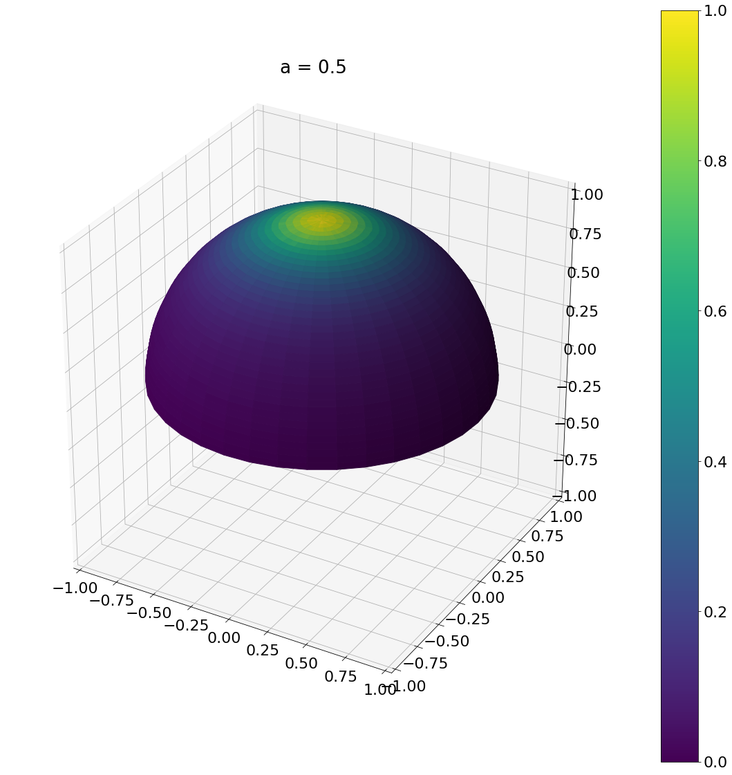
a = beckmann_width_to_phong(0.5)
theta, phi = sample_phong_normal(a,N)
ax = hemisphereheatmap(theta,phi,hemi_res)
ax.set_title(f"a = {a}")
plt.show()
a = beckmann_width_to_phong(1)
theta, phi = sample_phong_normal(a,N)
ax = hemisphereheatmap(theta,phi,hemi_res)
ax.set_title(f"a = {a}")
plt.show()


Algorithm
Sample microfacet normal according to the Phong distribution:
- Choose uniform numbers \(u_1, u_2\) in \([0,1]\)
- Calculate \(\theta = \cos^{-1}(\sqrt[a_p+2]{1 - u_1} )\) or \(\theta = \cos^{-1}(\sqrt[a_p+2]{u_1} )\)
- Calculate \(\phi = 2\pi u_2\)
Optionally convert to cartesian coordinates with:
\[x = \sin\theta\cos\phi\] \[y = \sin\theta\sin\phi\] \[z = \cos\theta\]PDF Used In Monte Carlo Integration
\[p_m(\omega) = \frac{a_p +2}{2\pi}\cos^{a_p}\theta\cos\theta = \frac{a_p +2}{2\pi}\cos^{a_p+1}\theta\] \[p_m(\theta,\phi) = \frac{a_p +2}{2\pi}\cos^{a_p}\theta\cos\theta\sin\theta = \frac{a_p +2}{2\pi}\cos^{a_p +1}\theta\sin\theta\]Derivation
This distribution is just a special case of the power cosine hemisphere cap above, but with \(\theta_{max}=\frac{\pi}{2}, n = a_p+1\)
\[p(\omega) = \frac{n+1}{2\pi(1 - \cos^{n+1}\theta_{max}) }\cos^n\theta = \frac{n+1}{2\pi }\cos^n\theta=\frac{a_p+2}{2\pi }\cos^{a_p + 1}\theta\]The formula given by Walter et al. comes from replacing \(1-u_1\) by \(u_1\), since both are uniformly distributed within \([0,1]\).
Trowbridge–Reitz / GGX Distribution
The normals of the microfacets are distributed according to the Trowbridge–Reitz / GGX distribution:
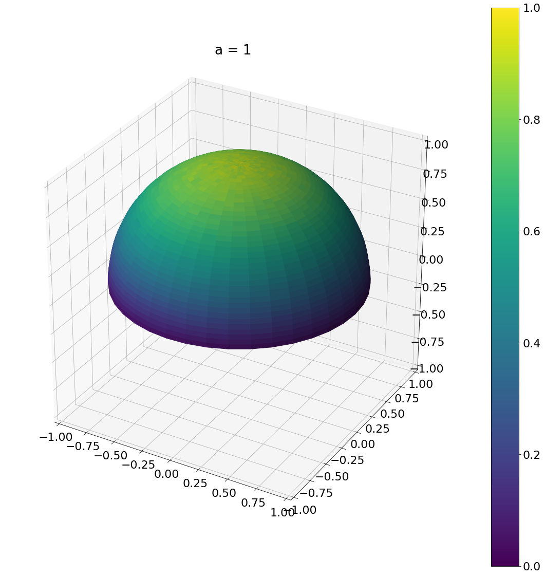
\[\begin{aligned} \operatorname{D}(\omega) &= \frac{a_g^2}{\pi\cos^4\theta (a_g^2 + \tan^2\theta)^2}\\ \operatorname{D}(\theta,\phi) &= \frac{a_g^2}{\pi\cos^4\theta (a_g^2 + \tan^2\theta)^2}\sin\theta \end{aligned}\]Here is the result:
def sample_ggx(a,N):
    u_1 = np.random.rand(N)
    u_2 = np.random.rand(N)

    theta = np.arctan(np.sqrt(a*a*u_1 /(1 - u_1)))
    phi = u_2*np.pi*2

    return theta,phi
theta, phi = sample_ggx(0.1,N)
ax = hemisphereheatmap(theta,phi,hemi_res)
ax.set_title("a = 0.1")

plt.show()

theta, phi = sample_ggx(0.5,N)
ax = hemisphereheatmap(theta,phi,hemi_res)
ax.set_title("a = 0.5")

plt.show()

theta, phi = sample_ggx(1,N)
ax = hemisphereheatmap(theta,phi,hemi_res)
ax.set_title("a = 1")
plt.show()

Algorithm
Sample microfacet normal according to the Trowbridge–Reitz / GGX distribution:
- Choose uniform numbers \(u_1, u_2\) in \([0,1]\)
- Calculate \(\theta = \tan^{-1}(\frac{a_g\sqrt{u_1}}{\sqrt{1- u_1}})\)
- Calculate \(\phi = 2\pi u_2\)
Optionally convert to cartesian coordinates with:
\[x = \sin\theta\cos\phi\] \[y = \sin\theta\sin\phi\] \[z = \cos\theta\]PDF Used In Monte Carlo Integration
\[p_m(\omega) = \frac{a_g^2\cos\theta}{\pi\cos^4\theta (a_g^2 + \tan^2\theta)^2} = \frac{a_g^2}{\pi\cos^3\theta (a_g^2 + \tan^2\theta)^2}\] \[p_m(\theta,\phi) = \frac{a_g^2\cos\theta\sin\theta}{\pi\cos^4\theta (a_g^2 + \tan^2\theta)^2}= \frac{a_g^2\tan\theta}{\pi\cos^2\theta (a_g^2 + \tan^2\theta)^2}\]Derivation
Due to normalization, the densities are given as follows:
\[\begin{aligned} p(\omega) &= D(\omega)\cos\theta\\ p(\theta,\phi) &= p(\omega)\sin\theta\\ &= \frac{a_g^2\cos\theta\sin\theta}{\pi\cos^4\theta (a_g^2 + \tan^2\theta)^2}\\ &= \frac{a_g^2\tan\theta}{\pi\cos^2\theta (a_g^2 + \tan^2\theta)^2} \end{aligned}\]Marginal And Conditional Densities:
\[\begin{aligned} p_\theta(\theta) &= \int_0^{2\pi}p(\theta,\phi)d\phi \\ &=\int_0^{2\pi}\frac{a_g^2\tan\theta}{\pi\cos^2\theta (a_g^2 + \tan^2\theta)^2} d\phi \\ &= 2\pi\frac{a_g^2\tan\theta}{\pi\cos^2\theta (a_g^2 + \tan^2\theta)^2}\\ &= 2a_g^2\frac{\tan\theta}{\cos^2\theta (a_g^2 + \tan^2\theta)^2}\\ &= 2\pi p(\theta, \phi) \end{aligned}\] \[p(\phi \vert \theta) = \frac{p(\theta,\phi)}{p_\theta(\theta)} = \frac{p(\theta,\phi)}{2\pi p(\theta,\phi)} = \frac{1}{2\pi}\]Compute CDFs
\[P_\theta(\theta) = \int_{0}^{\theta}2a_g^2\frac{\tan\theta'}{\cos^2\theta' (a_g^2 + \tan^2\theta')^2}d\theta'\]To solve this integral, we change variables and introduce \(u = \tan\theta'\). That gives us \(du = (\tan\theta')'d\theta' = \frac{1}{\cos^2\theta'}d\theta'\). Solving for \(d\theta'\) (with the usual slight abuse of notation): \(d\theta' = \cos^2\theta' du\).
As we will resubstitute later, for now let’s disregard the limits:
\[\begin{aligned} P_\theta(\theta) &= \int 2a_g^2\frac{\tan\theta'}{\cos^2\theta' (a_g^2 + \tan^2\theta')^2}d\theta' \\ &= 2a_g^2 \int \frac{u}{\cos^2\theta' (a_g^2 + u^2)^2}\cos^2\theta'du\\ &= 2a_g^2 \int \frac{u}{(a_g^2 + u^2)^2} du\\ \end{aligned}\]We will do a second substitution: \(v = a_g^2 + u^2\). That gives us \(dv = (a_g^2 +u^2)'du = 2udu\). Solving for \(du\): \(du = \frac{dv}{2u}\)
\[\begin{aligned} 2a_g^2 \int \frac{u}{(a_g^2 + u^2)^2} du &= 2a_g^2 \int \frac{u}{v^2} \frac{dv}{2u} \\ &= a_g^2 \int \frac{1}{v^2} dv \end{aligned}\]This can be easily solved:
\[\begin{aligned} a_g^2 \int \frac{1}{v^2} dv \\ &= a_g^2 [-\frac{1}{v}] \\ &= -a_g^2 [\frac{1}{v}] \end{aligned}\]Resubstituting \(v = a_g^2 + u^2\):
\[\begin{aligned} -a_g^2 [\frac{1}{v}] &= -a_g^2 [\frac{1}{a_g^2 + u^2}] \end{aligned}\]Resubstituting \(u = \tan\theta'\):
\[\begin{aligned} P_\theta(\theta) &= -a_g^2 [\frac{1}{a_g^2 + u^2}]\\ &= -a_g^2 [\frac{1}{a_g^2 + \tan^2\theta'}]_0^{\theta}\\ &= -a_g^2 (\frac{1}{a_g^2 + \tan^2\theta} - \frac{1}{a_g^2 + \tan^20})\\ &= -a_g^2 (\frac{1}{a_g^2 + \tan^2\theta} - \frac{1}{a_g^2})\\ &= 1 - \frac{a_g^2}{a_g^2 + \tan^2\theta} \end{aligned}\] \[P(\phi \vert \theta) = \int_{0}^{\phi}p(\phi ' \vert \theta)d\phi' = \int_{0}^{\phi} \frac{1}{2\pi}d\phi' =\frac{\phi}{2\pi}\]Invert CDFs
\[\begin{aligned} u_1 &= P_\theta(\theta)\\ &= 1 - \frac{a_g^2}{a_g^2 + \tan^2\theta} \\ u_1 - 1&=- \frac{a_g^2}{a_g^2 + \tan^2\theta} \\ 1- u_1 &= \frac{a_g^2}{a_g^2 + \tan^2\theta} \\ a_g^2 + \tan^2\theta &= \frac{a_g^2}{1- u_1} \\ \tan^2\theta &= \frac{a_g^2}{1- u_1} -a_g^2 \\ \tan\theta &= \sqrt{\frac{a_g^2}{1- u_1} -a_g^2}\\ \theta &= \tan^{-1}(\sqrt{\frac{a_g^2}{1- u_1} -a_g^2}) \\ &= \tan^{-1}(\sqrt{\frac{a_g^2 - a_g^2(1-u_1)}{1- u_1}}) \\ &= \tan^{-1}(\sqrt{\frac{a_g^2- a_g^2+ a_g^2u_1}{1- u_1}}) \\ &= \tan^{-1}(\sqrt{\frac{a_g^2u_1}{1- u_1}}) \\ &= \tan^{-1}(\frac{a_g\sqrt{u_1}}{\sqrt{1- u_1}}) \end{aligned}\]Here the last line is the formulation found in Walter et al.
\[\begin{aligned} u_2 &= P(\phi \vert \theta) \\ &= \frac{\phi}{2\pi}\\ \phi &= u_22\pi \end{aligned}\]