Simple proofs for some basic distancefield properties
I’m currently working a lot with distancefields. Distancefields can be described pretty easily. Given some kind of object, a distancefield (\(s\)) will tell you for every point in space, how far away the next point of an object is. The first thing to note is, that the object can now characterized by all points in space, for which the distance is zero.
If you have a closed object, you can use a distancefield for its surface and add a sign to get a signed distancefield. Depending on convention, the inside of an object will have a negative or positive sign and the outside the opposite. This gives us an easy method to check, whether a point is inside or outside.
While this is simple enough, there are a few properties of interest. These are used a lot of times, but it’s really hard to find any resources justifying them besides appealing to intuition or similar things. So I want to show some easy to understand explanations why these properties are valid. Keep in mind, that I will try to avoid some special case details as they would distract from the general idea (and are not that hard to take care of). First some notations that I will use and then the properties:
\(s : \mathbb{R}^n \rightarrow \mathbb{R}\): Distancefield
\(\nabla s\): Gradient of the distancefield
\(\mathbf{C}\): Closest point on the surface
\(\mathbf{P}\): Arbitrary point in space
\(\mathbf{v} = \mathbf{P} - \mathbf{C}\):
Vector connecting \(\mathbf{C}\) and \(\mathbf{P}\)
With that, now the properties, which will be explained in more detail when they come up:
- \(\mathbf{P}_t = \mathbf{C} + t\mathbf{v}, t \in [0,1] \Rightarrow\): \(\mathbf{C}\) is the closest surface point
- \[\nabla s(\mathbf{P}) \parallel \mathbf{v}\]
- \[\left\lVert\nabla s(\mathbf{P})\right\rVert = 1\]
- \[\mathbf{C} = \mathbf{P} - s(\mathbf{P})\nabla s(\mathbf{P})\]
We start with Property 1:
\(\mathbf{P}_t = \mathbf{C} + t\mathbf{v}, t \in [0,1] \Rightarrow\): \(\mathbf{C}\) is the closest surface point
This means, that if we take any point on the line connecting \(\mathbf{C}\) and \(\mathbf{P}\), then \(\mathbf{C}\) will still be the closest surface point. This is actually easy to see. Let’s look at an example:
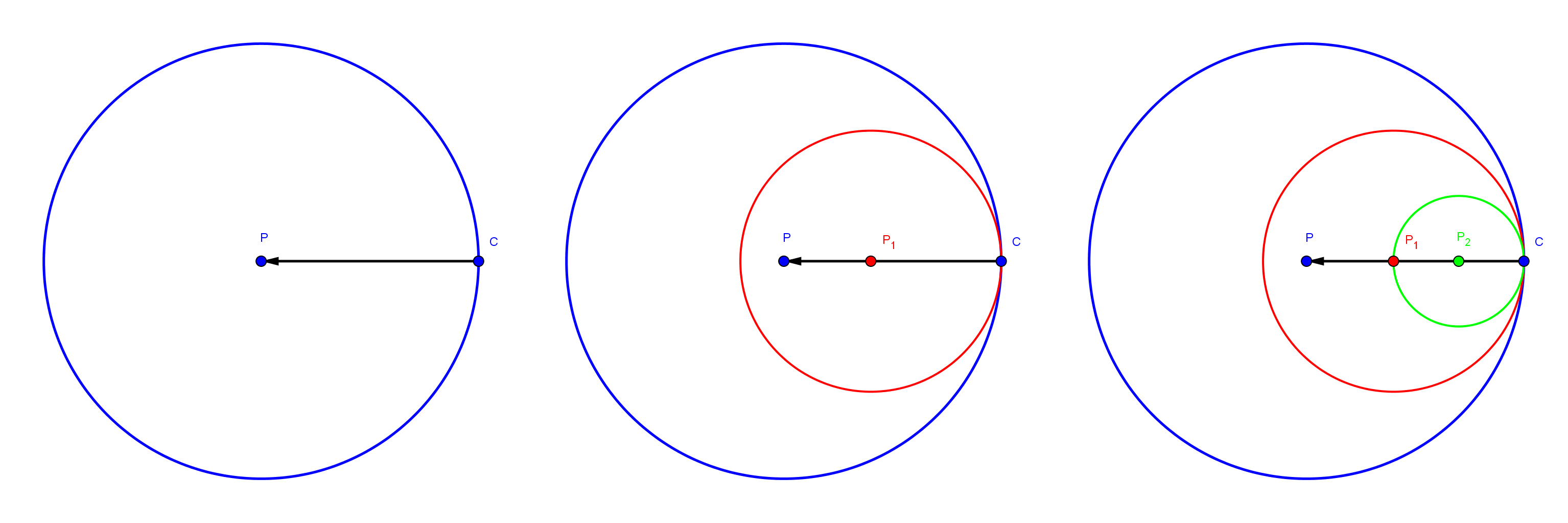
Left we see the line connecting \(\mathbf{C}\) and \(\mathbf{P}\), with the latter one being in the center. Since we know, that \(\mathbf{C}\) is the closest point, there can’t be any other point closer than that distance. That free region is marked with a circle. We now add two points on the line. Since we know, that \(\mathbf{C}\) is a surface point, we can use the distance to it as a starting point and draw circles with radius equal to that distance around them. If any point was closer than \(\mathbf{C}\), that point would need to lie inside of that circle. But the circles of the line points are contained in the one of \(\mathbf{P}\). Since we know, that no other surface point lies in the bigger circle, we know that there can’t be one in the smaller ones. Therefore \(\mathbf{C}\) is the closest point to any point on the line. In 3D or any other dimension, we just have to replace the circle with a sphere (a 2D sphere is just a circle, a 1D sphere is a line segment…)
Property 2:
\[\nabla s(\mathbf{P}) \parallel \mathbf{v}\]This property says, that the gradient of the distancefield \(s\) at \(\mathbf{P}\) is parallel to the connecting vector \(\mathbf{v}\). The gradient is the vector of all partial derivatives. So for a 2D field, the distancefield will also be 2D (same for any dimension). One important property of the gradient is, that it will point in the direction of greatest increase. So if we find that direction, we know where the gradient points to! For that, we use the following setup:
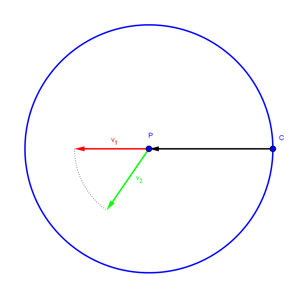
We take two vectors with the same length \(\mathbf{v}_1\) and \(\mathbf{v}_2\). \(\mathbf{v}_1\) points along \(\mathbf{v}\). Since \(\mathbf{C}\) is still the closest point (we choose a length that is smaller than the closest point outside of the circle) we can find the value of the distancefield by computing the length from \(\mathbf{C}\) to \(\mathbf{Q}_1\) and \(\mathbf{Q}_2\). So we have the following setup:
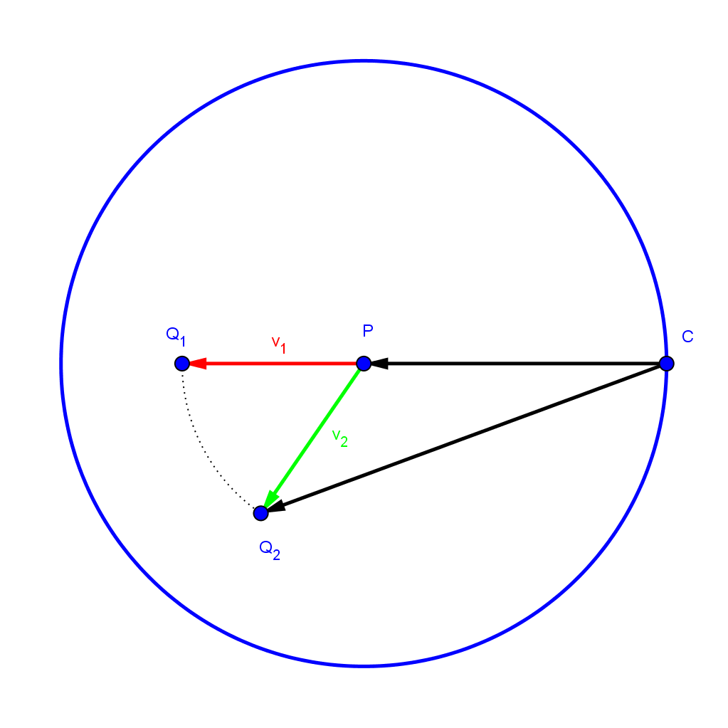
The length from \(\mathbf{C}\) to \(\mathbf{Q}_1\) ist just the length of \(\mathbf{v}\) plus the length of \(\mathbf{v}_1\), since the point in the same direction creating one line. We can now show, that \(\mathbf{v}_1\) is the direction of greatest increase.
\[\left\lVert \mathbf{v} \right\rVert +\left\lVert \mathbf{v}_1 \right\rVert = \left\lVert \mathbf{v} \right\rVert +\left\lVert \mathbf{v}_2 \right\rVert > \left\lVert \mathbf{v} +\mathbf{v}_2 \right\rVert\]That’s it! The first step follows from the fact, that both direction vectors have the same length. The second inequality is the basic triangle inequality, the sum of two sides is always longer than the last side (you could also use some vector algebra and just compute the dot product). The two last quantities would be the same only if \(\mathbf{v}_2\) and \(\mathbf{v}_1\) were the same.
Property 3:
\[\left\lVert\nabla s(\mathbf{P})\right\rVert = 1\]The length of the gradient of the distancefield is 1, meaning we always get a normalized vector! For this we use another property of the gradient, namely the directional derivative. The directional derivative can be expressed with a unit direction and the gradient. In general for a unit vector \(\mathbf{u}\) we have:
\[\lim_{h\rightarrow 0} \frac{s(\mathbf{P} + h\mathbf{u}) - s(\mathbf{P})}{h} = \nabla s(\mathbf{P})\cdot \mathbf{u} = \left\lVert\nabla s(\mathbf{P})\right\rVert \left\lVert\mathbf{u}\right\rVert \cos \alpha = \left\lVert\nabla s(\mathbf{P})\right\rVert \cos \alpha\]The last line follows from the fact that \(\mathbf{u}\) is a unit vector. If we now choose a vector with the same direction as the gradient, then the angle between them will be zero and the cosine term one. We already know the direction of the gradient, it is along \(\mathbf{v}\). So let \(\hat{\mathbf{v}}\) be the unit vector in the direction of \(\mathbf{v}\). Then we have:
\[\lim_{h\rightarrow 0} \frac{s(\mathbf{P} + h\hat{\mathbf{v}}) - s(\mathbf{P})}{h} = = \left\lVert\nabla s(\mathbf{P})\right\rVert\]So if we know the directional derivative in direction of \(\hat{\mathbf{v}}\), then we know the magnitude of the gradient! But we can compute that derivative very easily by noting the fact, that the distance at a distance \(h\) along \(\hat{\mathbf{v}}\) is just \(h\) more than the distance at \(\mathbf{P}\) (for small values of \(h\) which are less than the distance to a point outside of the circle, but that’s a technicality): \(s(\mathbf{P} + h\hat{\mathbf{v}}) = s(\mathbf{P}) + h\). Putting that in the above equation:
\[\begin{aligned} \lim_{h\rightarrow 0} \frac{s(\mathbf{P} + h\hat{\mathbf{v}}) - s(\mathbf{P})}{h} &= \lim_{h\rightarrow 0} \frac{s(\mathbf{P}) + h - s(\mathbf{P})}{h} \\ &= \lim_{h\rightarrow 0}\frac{h}{h} \\ &= 1 \end{aligned}\]So the result is, that the length of the gradient is exactly one!
Property 4
\[\mathbf{C} = \mathbf{P} - s(\mathbf{P})\nabla s(\mathbf{P})\]This says, that we can reconstruct the closest point at \(\mathbf{P}\) with the distancefield and its gradient. This pretty much follows from the above properties. We know that \(\mathbf{C}\) lies in the opposite direction of \(\mathbf{v}\) (by definition). We also know, that the length of \(\mathbf{v}\) is just the distance from \(\mathbf{C}\) to \(\mathbf{P}\), given by \(s(\mathbf{P})\) (also by defintion). Therefore, we get to \(\mathbf{C}\) by adding \(-\mathbf{v}\) to \(\mathbf{P}\). By property 2, we know that the gradient is parallel to \(\mathbf{v}\). By property 3 we know, that the gradient is a unit vector. Therefore \(\mathbf{v} = s(\mathbf{P})\nabla s(\mathbf{P})\). By property 1, we can travel along \(\mathbf{v}\) without getting to a point, where \(\mathbf{C}\) is not the closest point. So putting this all together:
\[\begin{aligned} \mathbf{C} &= \mathbf{P} - \mathbf{v} \\ &= \mathbf{P} - s(\mathbf{P})\nabla s(\mathbf{P}) \end{aligned}\]This was all, thanks for reading :)